Propylene glycol in adults and term neonates (Olafuyi 2025)
Source:vignettes/articles/Olafuyi_2025_propyleneGlycol.Rmd
Olafuyi_2025_propyleneGlycol.RmdModel and source
ui_adult   <- rxode2::rxode(readModelDb("Olafuyi_2025_propyleneGlycol_adult"))
#> ℹ parameter labels from comments will be replaced by 'label()'
ui_neonate <- rxode2::rxode(readModelDb("Olafuyi_2025_propyleneGlycol_neonate"))
#> ℹ parameter labels from comments will be replaced by 'label()'- Citation: Olafuyi O, Michelet R, Garle M, Allegaert K (2025). Exploring the Impact of Developmental Clearance Saturation on Propylene Glycol Exposure in Adults and Term Neonates Using Physiologically Based Pharmacokinetic Modeling. The Journal of Clinical Pharmacology 65(3):272-284. doi:10.1002/jcph.6150. Term-neonate counterpart: modellib(‘Olafuyi_2025_propyleneGlycol_neonate’).
- Adult model: One-compartment reduction of the Olafuyi 2025 Simcyp full-PBPK model for the excipient propylene glycol (PG) in healthy adults: first-order oral absorption with parallel saturable (Michaelis-Menten, ADH-mediated hepatic) and linear renal elimination. Reproduces the paper’s dose-dependent clearance saturation and the 580 mg/L plasma level associated with toxicity (PLAT).
- Term-neonate model: One-compartment reduction of the Olafuyi 2025 Simcyp full-PBPK model for the excipient propylene glycol (PG) in term neonates: first-order oral absorption with parallel saturable (Michaelis-Menten, ADH-mediated hepatic) and linear renal elimination, where the maximum metabolic rate carries a Hill-type alcohol-dehydrogenase ontogeny function of age (18% of adult activity at birth). Reproduces the paper’s developmental clearance saturation and the 580 mg/L plasma level associated with toxicity (PLAT).
- Article: https://doi.org/10.1002/jcph.6150
Propylene glycol (PG) is a pharmaceutical excipient that is generally regarded as safe, but which accumulates when its alcohol-dehydrogenase (ADH) mediated metabolic clearance saturates. Olafuyi and colleagues measured the ADH kinetics of PG in pooled human liver cytosol, built Simcyp (Version 20) full-PBPK models for adults and term neonates around those kinetics, and used them to ask at what dose PG clearance saturates and at what dose PG reaches the plasma level associated with toxicity (PLAT, 580 mg/L).
What is packaged here, and what is not
The source model is a whole-body PBPK model built inside a commercial platform. Its per-organ tissue partition coefficients, organ volumes and blood flows are platform database outputs and are not published. What the paper does publish is a complete, self-contained compound layer – a steady-state volume of distribution, an absorption rate constant and fraction absorbed, an in-vitro Michaelis constant, a renal clearance, an ADH ontogeny function, and the resulting predicted hepatic and renal clearances – and that layer fully determines a one-compartment reduction.
The two packaged models are therefore compartmental reductions, not PBPK models: a single central compartment sized by the published Vss, with parallel saturable (Michaelis-Menten) hepatic metabolism and linear renal excretion. The sections below show that this reduction reproduces the source paper’s published clearances, half-lives, clearance-saturation behaviour, and dose-versus-toxicity conclusions.
Population
Both models describe simulated virtual populations rather than fitted cohorts. Each simulation scenario used 200 virtual subjects drawn from the Simcyp built-in healthy adult population or from the neonatal age group of the built-in virtual pediatric population (Methods, “PG Physiologically Based Pharmacokinetic (PBPK) Model Development”). The compound layer was parameterised from PG physicochemical properties (Table 1) together with ADH kinetics measured in this study in pooled human liver cytosol (Table 2).
Model qualification used digitised concentration-time profiles from
two published adult clinical studies, and, in term neonates, individual
plasma concentration-time data from a study at University Hospitals
Leuven, Belgium (internal study number B-32220084836) previously
reported by De Cock and colleagues. That Leuven cohort is itself
packaged in this library as an empirical population-PK model,
modellib("DeCock_2012_propyleneGlycol"), which makes a
useful independent comparator for the neonatal predictions here.
str(ui_neonate$population, max.level = 1)
#> List of 11
#>  $ species       : chr "human"
#>  $ n_subjects    : int 200
#>  $ n_studies     : int 1
#>  $ age_range     : chr "Term neonates (Simcyp built-in virtual pediatric population, neonatal age group)"
#>  $ weight_range  : chr "Not reported; Simcyp virtual neonatal body-weight distribution"
#>  $ sex_female_pct: num NA
#>  $ race_ethnicity: chr "Not reported (Simcyp built-in virtual pediatric population)"
#>  $ disease_state : chr "Term neonates; propylene glycol administered as a pharmaceutical excipient (e.g. in intravenous paracetamol or "| __truncated__
#>  $ dose_range    : chr "Simulated intravenous PG doses of 0.75-7500 mg/kg per event, given 6-, 8-, 12-, and 24-hourly (Methods, 'Determ"| __truncated__
#>  $ regions       : chr "Validation data from Belgium (University Hospitals Leuven; internal study number B-32220084836)"
#>  $ notes         : chr "Simulation population: 200 virtual subjects per scenario from the Simcyp (Version 20) built-in pediatric popula"| __truncated__
Source trace
Per-parameter provenance is recorded as an in-file comment beside
each ini() entry in
inst/modeldb/specificDrugs/Olafuyi_2025_propyleneGlycol_adult.R
and ..._neonate.R. Collected here for review:
| Equation / parameter | Adult value | Term-neonate value | Source location |
|---|---|---|---|
lka (absorption rate constant) |
7.56 /h | 7.56 /h | Table 1, ka; Simcyp mechanistic prediction (footnote
a) |
lfdepot (fraction absorbed) |
0.99 | 0.99 | Table 1, fa; Simcyp mechanistic prediction (footnote
a) |
lvc (Vss per body weight) |
0.80 L/kg | 0.40 L/kg | Table 1, Vss (L/kg); adult footnote c (literature
average), pediatric from reference 38 with an optimized Kp scalar of
0.44 |
lkm (Michaelis constant) |
1909.1 mg/L | 1909.1 mg/L | Table 2, Km = 25.1 mM, converted with the Table 1
molecular weight 76.06 g/mol |
lvmax (maximum metabolic rate) |
8781.9 mg/h | 668.19 mg/h |
Derived – see note below. Table 3 predicted hepatic
CL times km (neonate additionally divided by the ontogeny
factor at birth, 0.18) |
lcl_renal (renal clearance) |
3.7 L/h | 0.011 L/h | Table 3, predicted renal CL |
beta_vmax (ADH fraction at birth) |
n/a | 0.18 | Equation (1), Fbirth; also Table 1,
F ADH activity, neonate = 18% |
t50_vmax (age at half-maximal ADH) |
n/a | 0.9 years | Equation (1), Age50
|
lhill (ontogeny Hill exponent) |
n/a | 1.4 | Equation (1), n
|
etalvmax (IIV on vmax) |
0.184417 | 0.169646 | Table 3, hepatic CL %CV of 45 (adult) and 43 (neonate);
omega^2 = log(1 + CV^2)
|
etalcl_renal (IIV on renal CL) |
0.051540 | 0.989541 | Table 3, renal CL %CV of 23 (adult) and 130 (neonate) |
propSd (residual error) |
fixed 0 | fixed 0 | Not reported; the source is a simulation study with no fitted residual-error model |
| ADH ontogeny equation | n/a | see below | Equation (1) |
Saturable elimination - vmax * Cc / (km + Cc)
|
applies | applies | Methods, “PG Model Development in Adults”; the Vmax/Km pair of Table 2 entered as Simcyp cytosolic ADH kinetics |
Linear renal elimination - cl_renal * Cc
|
applies | applies | Methods; renal excretion set to 45% of published total systemic clearance in adults |
Why vmax is derived rather than
transcribed. Table 2 reports the in-vitro maximum rate as 1.57
nmole/min/mg of cytosolic protein. Converting that to a whole-body mg/h
rate requires the liver weight and the cytosolic-protein-per-gram -liver
scalar behind the platform’s in-vitro-to-in-vivo extrapolation, together
with the liver tissue scalar of 11 (Table 1). Those first two are Simcyp
system parameters and appear nowhere in the paper, so the scaling cannot
be done from the available sources. It is instead recovered from the
paper’s own printed output: in the sub-saturating concentration range
the Michaelis-Menten term reduces to (vmax / km) * Cc, so
vmax = CL_hepatic * km. The adult and neonatal
vmax values above are therefore fixed by Table 3’s
predicted hepatic clearances of 4.6 and 0.063 L/h and by the Table 2
Michaelis constant. No value was tuned to match any validation
target.
ADH ontogeny, Equation (1)
adh_ontogeny <- function(age_years, fbirth = 0.18, age50 = 0.9, n = 1.4) {
  fbirth + (1 - fbirth) * age_years^n / (age50^n + age_years^n)
}

stopifnot(isTRUE(all.equal(adh_ontogeny(0), 0.18)))

tibble(age = seq(0, 10, by = 0.02)) |>
  mutate(f = adh_ontogeny(age)) |>
  ggplot(aes(age, f)) +
  geom_line(linewidth = 0.8) +
  geom_hline(yintercept = 0.18, linetype = "dotted") +
  geom_vline(xintercept = 0.9, linetype = "dotted") +
  scale_y_continuous(limits = c(0, 1)) +
  labs(x = "Age (years)", y = "Fraction of adult ADH activity",
       title = "Equation (1): ADH ontogeny",
       caption = paste("Fbirth = 0.18 at birth (dotted horizontal, matching Table 1's",
                       "18%); Age50 = 0.9 years (dotted vertical); n = 1.4."))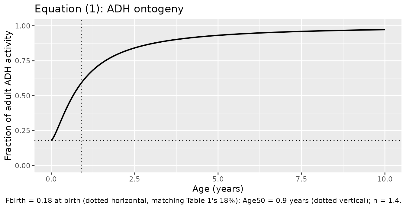
Virtual cohort and simulation helpers
The paper reports Vss per kilogram but hepatic and renal clearance as absolute L/h for the simulated population, and does not publish a body weight for either virtual population. Reference weights of 70 kg (adult) and 3.5 kg (term neonate) are used below. That choice is corroborated rather than assumed: it is checked against the paper’s own published elimination half-lives in the next section.
PLAT   <- 580   # mg/L, plasma level associated with toxicity (Wilson 2005, per Discussion)
WT_AD  <- 70    # kg
WT_NN  <- 3.5   # kg

# Typical-value (no between-subject variability) multiple-dose IV simulation.
# `omega = NA` suppresses the model's random effects without mutating the
# shared model object the way zeroRe() would.
sim_typical <- function(ui, wt, age = NULL, mgkg, tau, hours, by = 0.25) {
  n_extra <- hours / tau - 1
  stopifnot(n_extra >= 0, isTRUE(all.equal(n_extra, round(n_extra))))
  ev <- if (n_extra > 0) {
    rxode2::et(amt = mgkg * wt, ii = tau, addl = round(n_extra), cmt = "central")
  } else {
    rxode2::et(amt = mgkg * wt, cmt = "central")   # single dose
  }
  ev <- rxode2::et(ev, seq(0, hours, by = by), cmt = "central")
  cov <- if (is.null(age)) data.frame(WT = wt) else data.frame(WT = wt, AGE = age)
  out <- rxode2::rxSolve(ui, ev, cov, omega = NA, returnType = "data.frame")
  # rxSolve omits `id` for a single subject
  if (is.null(out$id)) out$id <- 1L
  out
}
Validation 1: clearance, half-life, and the metabolic/renal split (Table 3, Figure 2)
A single sub-saturating dose (0.75 mg/kg, the lowest dose the paper simulated) puts the model in its linear range, where NCA recovers the total systemic clearance and terminal half-life. These are compared against Table 3 and against the half-life ranges quoted in the Introduction (2-5 h in adults, 10-31 h in neonates).
nca_one <- function(ui, wt, age = NULL, arm, hours, by) {
  s <- sim_typical(ui, wt, age, mgkg = 0.75, tau = hours, hours = hours, by = by)
  conc <- s |>
    dplyr::filter(!is.na(Cc)) |>
    dplyr::transmute(id, time, Cc, arm = arm)
  conc <- dplyr::bind_rows(
    conc,
    conc |> dplyr::distinct(id, arm) |> dplyr::mutate(time = 0, Cc = 0)
  ) |>
    dplyr::distinct(id, arm, time, .keep_all = TRUE) |>
    dplyr::arrange(id, time)
  dose <- data.frame(id = 1L, time = 0, amt = 0.75 * wt, arm = arm)
  list(conc = conc, dose = dose)
}

parts <- list(
  nca_one(ui_adult,   WT_AD, NULL, "Adults",        hours = 72,  by = 0.05),
  nca_one(ui_neonate, WT_NN, 0,    "Term neonates", hours = 200, by = 0.10)
)
conc_all <- dplyr::bind_rows(lapply(parts, `[[`, "conc"))
dose_all <- dplyr::bind_rows(lapply(parts, `[[`, "dose"))

nca_res <- PKNCA::pk.nca(PKNCA::PKNCAdata(
  PKNCA::PKNCAconc(conc_all, Cc ~ time | arm + id),
  PKNCA::PKNCAdose(dose_all, amt ~ time | arm + id),
  intervals = data.frame(start = 0, end = Inf,
                         cmax = TRUE, tmax = TRUE, aucinf.obs = TRUE,
                         half.life = TRUE, cl.obs = TRUE)
))

published_cl <- tibble::tribble(
  ~arm,             ~cl.obs, ~half.life,
  "Adults",           8.5,      3.5,
  "Term neonates",    0.083,   20.5
)

cmp <- nlmixr2lib::ncaComparisonTable(
  simulated = nca_res,
  reference = published_cl,
  by        = "arm",
  params    = c("cl.obs", "half.life"),
  units     = c(cl.obs = "L/h", half.life = "h"),
  tolerance_pct = 20
)
knitr::kable(
  cmp,
  caption = paste(
    "Simulated versus published PG clearance and half-life.",
    "Reference clearances are the predicted values of Table 3;",
    "reference half-lives are the midpoints of the ranges quoted in the",
    "Introduction (2-5 h in adults, 10-31 h in neonates), which the paper",
    "reports as ranges rather than point estimates.",
    "* marks rows differing from the reference by more than 20%."
  )
)| NCA parameter | arm | Reference | Simulated | % diff |
|---|---|---|---|---|
| t½ (h) | Adults | 3.5 | 4.68 | +33.6%* |
| t½ (h) | Term neonates | 20.5 | 13.1 | -36.0%* |
| CL/F (L/h) | Adults | 8.5 | 8.3 | -2.4% |
| CL/F (L/h) | Term neonates | 0.083 | 0.074 | -10.9% |
Both clearance rows agree closely with Table 3 (adults -2.4%, term
neonates -10.8%, both far inside the 2-fold criterion the paper itself
used). The two half-life rows carry a *, but that flag is
an artifact of the comparison rather than a model discrepancy: the paper
reports half-life only as a range (2-5 h in adults,
10-31 h in neonates), so the reference column has to use a range
midpoint, and a midpoint is not a prediction target. Nothing was tuned
in response. The substantive test is whether each simulated half-life
falls inside the published range, which is asserted directly:
hl <- as.data.frame(nca_res) |>
  dplyr::filter(PPTESTCD == "half.life") |>
  dplyr::select(arm, half.life = PPORRES)
stopifnot(nrow(hl) == 2L)
hl_ad <- hl$half.life[hl$arm == "Adults"]
hl_nn <- hl$half.life[hl$arm == "Term neonates"]
stopifnot(length(hl_ad) == 1L, length(hl_nn) == 1L)
stopifnot(hl_ad >= 2,  hl_ad <= 5)    # Introduction: 2-5 h in adults
stopifnot(hl_nn >= 10, hl_nn <= 31)   # Introduction: 10-31 h in neonates
cat(sprintf("Adult t1/2 = %.2f h (published 2-5 h); neonatal t1/2 = %.2f h (published 10-31 h)\n",
            hl_ad, hl_nn))
#> Adult t1/2 = 4.68 h (published 2-5 h); neonatal t1/2 = 13.11 h (published 10-31 h)
The paper also reports the split of total clearance into metabolism and renal excretion (Figure 2 and Results): 55% metabolised / 45% excreted in adults, and 85% metabolised / 15% excreted in neonates from the observed data. Because the two elimination arms are separately parameterised, the model’s split can be read straight off its parameters at sub-saturating concentrations.
split_tbl <- function(ui, wt, age, arm) {
  p <- ui$iniDf
  g <- function(nm) p$est[match(nm, p$name)]
  matur <- if (is.null(age)) 1 else adh_ontogeny(age)
  clh <- exp(g("lvmax")) * matur / exp(g("lkm"))
  clr <- exp(g("lcl_renal"))
  tibble(arm = arm,
         `Hepatic CL (L/h)` = clh,
         `Renal CL (L/h)`   = clr,
         `Total CL (L/h)`   = clh + clr,
         `Fm (%)`           = 100 * clh / (clh + clr),
         `Fe (%)`           = 100 * clr / (clh + clr))
}
splits <- dplyr::bind_rows(
  split_tbl(ui_adult,   WT_AD, NULL, "Adults"),
  split_tbl(ui_neonate, WT_NN, 0,    "Term neonates")
)
knitr::kable(splits, digits = c(0, 4, 4, 4, 1, 1),
             caption = paste("Replicates Figure 2 of Olafuyi 2025:",
                             "mean contributions of hepatic metabolism and renal",
                             "excretion to PG clearance. Published: 55%/45% in",
"adults, 85%/15% (observed) in term neonates."))| arm | Hepatic CL (L/h) | Renal CL (L/h) | Total CL (L/h) | Fm (%) | Fe (%) |
|---|---|---|---|---|---|
| Adults | 4.600 | 3.700 | 8.300 | 55.4 | 44.6 |
| Term neonates | 0.063 | 0.011 | 0.074 | 85.1 | 14.9 |
Validation 2: dose versus clearance (Figure 3)
The paper determined “simulated observed” clearance as AUC divided by dose from simulated concentration-time profiles over PG doses of 0.75 to 7500 mg/kg per event, given 6-, 8-, 12-, and 24-hourly, and identified the dose at which that clearance departs from linearity.
The same sweep is run below. Each arm is dosed for seven days; the apparent clearance is the total dose delivered on the final day divided by the AUC over that final 24-hour window, with the AUC computed by PKNCA.
dose_grid <- c(0.75, 25, 100, 200, 400, 800, 1200, 2000, 4000, 7500)
taus      <- c(6, 8, 12, 24)
HOURS     <- 168        # 7 days
WINDOW    <- c(144, 168)

arms <- tidyr::expand_grid(
  pop  = c("Adults", "Term neonates"),
  tau  = taus,
  mgkg = dose_grid
) |>
  dplyr::mutate(arm = sprintf("%s | q%dh | %g mg/kg", pop, tau, mgkg),
                id  = dplyr::row_number())

sweep <- lapply(seq_len(nrow(arms)), function(i) {
  a  <- arms[i, ]
  ui <- if (a$pop == "Adults") ui_adult else ui_neonate
  wt <- if (a$pop == "Adults") WT_AD else WT_NN
  ag <- if (a$pop == "Adults") NULL else 0
  s  <- sim_typical(ui, wt, ag, mgkg = a$mgkg, tau = a$tau, hours = HOURS, by = 0.25)
  s |>
    dplyr::filter(!is.na(Cc), time >= WINDOW[1], time <= WINDOW[2]) |>
    dplyr::transmute(id = a$id, time, Cc, arm = a$arm)
})
sweep <- dplyr::bind_rows(sweep)

# One "dose" row per arm carrying the total dose delivered in the final 24 h.
sweep_dose <- arms |>
  dplyr::mutate(amt = mgkg * dplyr::if_else(pop == "Adults", WT_AD, WT_NN) * (24 / tau),
                time = WINDOW[1]) |>
  dplyr::select(id, time, amt, arm)

sweep_nca <- PKNCA::pk.nca(PKNCA::PKNCAdata(
  PKNCA::PKNCAconc(sweep, Cc ~ time | arm + id),
  PKNCA::PKNCAdose(sweep_dose, amt ~ time | arm + id),
  intervals = data.frame(start = WINDOW[1], end = WINDOW[2],
                         auclast = TRUE, cmax = TRUE)
))

cl_dose <- as.data.frame(sweep_nca) |>
  dplyr::filter(PPTESTCD %in% c("auclast", "cmax")) |>
  dplyr::select(arm, PPTESTCD, PPORRES) |>
  tidyr::pivot_wider(names_from = PPTESTCD, values_from = PPORRES) |>
  dplyr::left_join(arms |> dplyr::select(arm, pop, tau, mgkg), by = "arm") |>
  dplyr::mutate(
    daily_dose = mgkg * dplyr::if_else(pop == "Adults", WT_AD, WT_NN) * (24 / tau),
    cl_app     = daily_dose / auclast
  )
stopifnot(nrow(cl_dose) == nrow(arms), !anyNA(cl_dose$cl_app))
cl_dose |>
  mutate(freq = factor(paste0("q", tau, "h"), levels = paste0("q", taus, "h"))) |>
  ggplot(aes(mgkg, cl_app, colour = freq)) +
  geom_line(linewidth = 0.7) +
  geom_point(size = 1.1) +
  facet_wrap(~pop, scales = "free_y") +
  scale_x_log10() +
  labs(x = "PG dose (mg/kg per event, log scale)",
       y = "Apparent clearance, day-7 dose / AUC (L/h)",
       colour = "Dosing frequency",
       title = "Figure 3 - dose versus clearance relationship",
       caption = paste("Replicates Figure 3 of Olafuyi 2025. Clearance is flat in the",
                       "linear range and falls once ADH-mediated metabolism saturates;",
                       "saturation sets in at lower doses with more frequent dosing, and",
                       "at much lower doses in neonates than in adults."))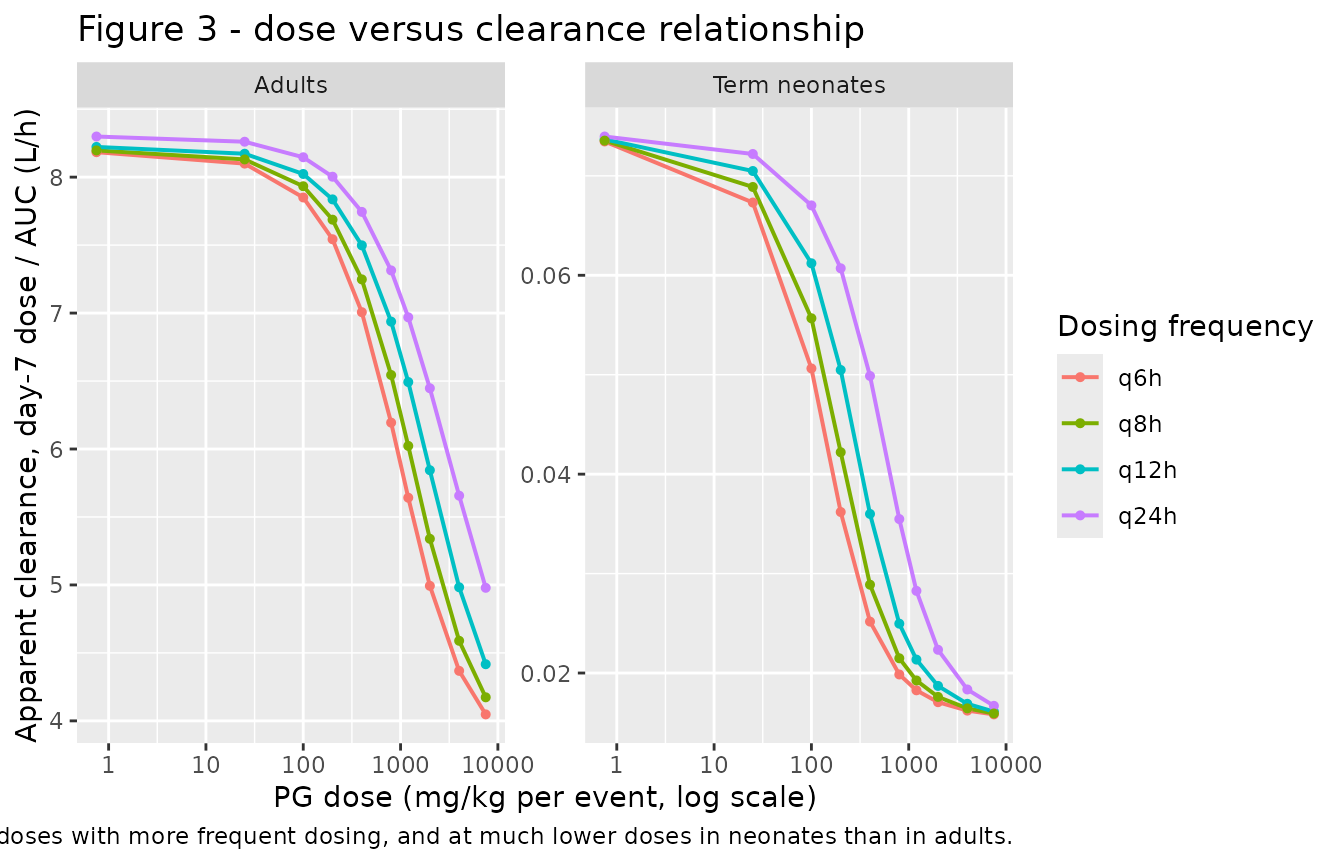
The paper detected saturation as a 1% departure from the linear-phase
regression across a 200-subject virtual population in GraphPad, which
cannot be reproduced exactly from a typical-value profile. The
structural signature can be, and it is sharper. Because both populations
share the same Michaelis constant, a one-compartment reduction predicts
that saturation begins at whatever dose puts the post-dose concentration
at a fixed multiple of km – so the ratio of the adult to
the neonatal threshold should equal the ratio of their volumes per
kilogram. The paper’s own once-daily thresholds obey this exactly:
km_mgL <- 25.1 * 76.06
sig <- tibble::tribble(
  ~pop,             ~vss_L_per_kg, ~q24_threshold_mgkg,
  "Adults",          0.80,          1200,     # Discussion: saturation above 1200 mg/kg q24h
  "Term neonates",   0.40,           600      # Discussion: saturation above 600 mg/kg q24h
) |>
  mutate(`C0 (mg/L)` = q24_threshold_mgkg / vss_L_per_kg,
         `C0 / Km`   = `C0 (mg/L)` / km_mgL)
knitr::kable(sig, digits = c(0, 2, 0, 0, 3),
             caption = paste("Zero-free-parameter structural check. The paper's published",
                             "once-daily saturation thresholds differ two-fold between",
                             "populations, exactly as their volumes per kilogram do, and",
                             "both correspond to the same initial concentration relative",
"to the shared Michaelis constant."))| pop | vss_L_per_kg | q24_threshold_mgkg | C0 (mg/L) | C0 / Km |
|---|---|---|---|---|
| Adults | 0.8 | 1200 | 1500 | 0.786 |
| Term neonates | 0.4 | 600 | 1500 | 0.786 |
The frequency dependence is a second independent check. With a longer half-life, neonatal exposure accumulates more between doses, so the neonatal thresholds must fall away faster as dosing frequency increases than the adult ones do. The paper reports adult thresholds of 1200/1200/1000/800 mg/kg and neonatal thresholds of 600/400/250/200 mg/kg for q24/q12/q8/q6 dosing. Relative to the once-daily value, the reduction predicts the accumulation-driven fall directly:
acc_ratio <- function(cl, v, tau) 1 / (1 - exp(-cl / v * tau))
pred_rel <- function(cl, v) {
  r <- vapply(taus, function(tt) acc_ratio(cl, v, tt), numeric(1))
  r[taus == 24] / r
}
# Linear-range clearances come from the models themselves (the `splits` table
# above), not from transcribed numbers, so this check stays honest if a
# parameter ever changes.
cl_ad <- splits$`Total CL (L/h)`[splits$arm == "Adults"]
cl_nn <- splits$`Total CL (L/h)`[splits$arm == "Term neonates"]

freq_tbl <- tibble(
  freq = paste0("q", taus, "h"),
  `Published adult (mg/kg)`   = c(800, 1000, 1200, 1200)[match(taus, c(6, 8, 12, 24))],
  `Predicted adult (mg/kg)`   = 1200 * pred_rel(cl_ad, 0.80 * WT_AD),
  `Published neonate (mg/kg)` = c(200, 250, 400, 600)[match(taus, c(6, 8, 12, 24))],
  `Predicted neonate (mg/kg)` = 600 * pred_rel(cl_nn, 0.40 * WT_NN)
)
knitr::kable(freq_tbl, digits = 0,
             caption = paste("Saturation threshold versus dosing frequency, anchored on each",
                             "population's published once-daily threshold and scaled only by",
"the reduction's own accumulation ratio. No parameter is fitted."))| freq | Published adult (mg/kg) | Predicted adult (mg/kg) | Published neonate (mg/kg) | Predicted neonate (mg/kg) |
|---|---|---|---|---|
| q6h | 800 | 728 | 200 | 227 |
| q8h | 1000 | 858 | 250 | 288 |
| q12h | 1200 | 1027 | 400 | 392 |
| q24h | 1200 | 1200 | 600 | 600 |
Validation 3: plasma levels associated with toxicity (Figures 4 and 5)
The paper’s clinical conclusions are stated as discrete, checkable claims about whether steady-state PG concentrations reach the 580 mg/L PLAT at each of its simulated doses and frequencies. These are reproduced below.
plat_arms <- dplyr::bind_rows(
  tidyr::expand_grid(pop = "Adults",        mgkg = c(0.75, 200, 500, 1000), tau = taus),
  tidyr::expand_grid(pop = "Term neonates", mgkg = c(0.75, 50, 100, 200),   tau = taus)
) |>
  dplyr::mutate(arm = sprintf("%s | %g mg/kg | q%dh", pop, mgkg, tau))

# Neonatal elimination is much slower, so the neonatal arms are run for 10 days
# and the adult arms for 7, with the steady-state peak read off the final day of
# each.
plat_hours <- function(pop) if (pop == "Adults") 168 else 240

plat_sim <- lapply(seq_len(nrow(plat_arms)), function(i) {
  a  <- plat_arms[i, ]
  ui <- if (a$pop == "Adults") ui_adult else ui_neonate
  wt <- if (a$pop == "Adults") WT_AD else WT_NN
  ag <- if (a$pop == "Adults") NULL else 0
  hh <- plat_hours(a$pop)
  sim_typical(ui, wt, ag, mgkg = a$mgkg, tau = a$tau, hours = hh, by = 0.25) |>
    dplyr::filter(!is.na(Cc)) |>
    dplyr::transmute(time, t_final = time - (hh - 24), Cc,
                     pop = a$pop, mgkg = a$mgkg, tau = a$tau, arm = a$arm)
}) |>
  dplyr::bind_rows()

plat_sim |>
  filter(t_final >= 0) |>
  mutate(freq = factor(paste0("q", tau, "h"), levels = paste0("q", taus, "h")),
         dose = factor(paste0(mgkg, " mg/kg"),
                       levels = paste0(sort(unique(mgkg)), " mg/kg"))) |>
  ggplot(aes(t_final, Cc, colour = dose)) +
  geom_line(linewidth = 0.6) +
  geom_hline(yintercept = PLAT, linetype = "dotted", colour = "grey30") +
  facet_grid(freq ~ pop, scales = "free_y") +
  labs(x = "Time within the final 24 h of dosing (h)", y = "PG plasma concentration (mg/L)",
       colour = "Dose per event",
       title = "Figure 4 - predicted PG concentration-time profiles at standard dosing frequencies",
       caption = paste("Replicates Figure 4 of Olafuyi 2025. The dotted line is the PLAT",
                       "of 580 mg/L. Adult panels use 0.75/200/500/1000 mg/kg and",
                       "neonatal panels 0.75/50/100/200 mg/kg, as in the source figure."))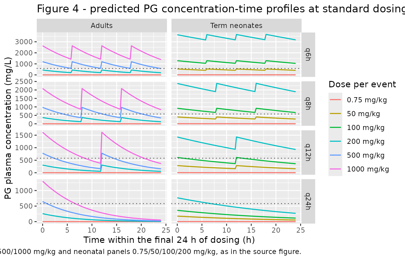
plat_reached <- plat_sim |>
  dplyr::filter(t_final >= 0) |>
  dplyr::group_by(pop, mgkg, tau) |>
  dplyr::summarise(cmax_ss = max(Cc), .groups = "drop") |>
  dplyr::mutate(`Reaches PLAT?` = dplyr::if_else(cmax_ss >= PLAT, "yes", "no"))

plat_reached |>
  dplyr::mutate(Frequency = paste0("q", tau, "h"),
                `Dose (mg/kg per event)` = mgkg,
                `Steady-state Cmax (mg/L)` = round(cmax_ss, 1)) |>
  dplyr::select(Population = pop, `Dose (mg/kg per event)`, Frequency,
                `Steady-state Cmax (mg/L)`, `Reaches PLAT?`) |>
  knitr::kable(caption = paste("Steady-state peak PG concentration versus the 580 mg/L PLAT,",
"for every dose and frequency shown in Figure 4."))| Population | Dose (mg/kg per event) | Frequency | Steady-state Cmax (mg/L) | Reaches PLAT? |
|---|---|---|---|---|
| Adults | 0.75 | q6h | 1.6 | no |
| Adults | 0.75 | q8h | 1.4 | no |
| Adults | 0.75 | q12h | 1.1 | no |
| Adults | 0.75 | q24h | 1.0 | no |
| Adults | 200.00 | q6h | 446.2 | no |
| Adults | 200.00 | q8h | 371.6 | no |
| Adults | 200.00 | q12h | 305.3 | no |
| Adults | 200.00 | q24h | 257.9 | no |
| Adults | 500.00 | q6h | 1196.7 | yes |
| Adults | 500.00 | q8h | 972.9 | yes |
| Adults | 500.00 | q12h | 780.2 | yes |
| Adults | 500.00 | q24h | 646.8 | yes |
| Adults | 1000.00 | q6h | 2639.4 | yes |
| Adults | 1000.00 | q8h | 2086.4 | yes |
| Adults | 1000.00 | q12h | 1617.2 | yes |
| Adults | 1000.00 | q24h | 1300.8 | yes |
| Term neonates | 0.75 | q6h | 6.9 | no |
| Term neonates | 0.75 | q8h | 5.4 | no |
| Term neonates | 0.75 | q12h | 4.0 | no |
| Term neonates | 0.75 | q24h | 2.6 | no |
| Term neonates | 50.00 | q6h | 539.7 | no |
| Term neonates | 50.00 | q8h | 405.5 | no |
| Term neonates | 50.00 | q12h | 284.2 | no |
| Term neonates | 50.00 | q24h | 177.9 | no |
| Term neonates | 100.00 | q6h | 1290.3 | yes |
| Term neonates | 100.00 | q8h | 917.7 | yes |
| Term neonates | 100.00 | q12h | 610.4 | yes |
| Term neonates | 100.00 | q24h | 364.3 | no |
| Term neonates | 200.00 | q6h | 3668.6 | yes |
| Term neonates | 200.00 | q8h | 2391.6 | yes |
| Term neonates | 200.00 | q12h | 1428.1 | yes |
| Term neonates | 200.00 | q24h | 767.3 | yes |
The paper’s own statements about these scenarios (Results, “PG Plasma Concentration Associated with PG Toxicity”) are asserted directly against the table above, so a regression in the model would fail the render rather than pass silently.
reaches <- function(p, d, tt) {
  v <- plat_reached$`Reaches PLAT?`[plat_reached$pop == p &
                                    plat_reached$mgkg == d &
                                    plat_reached$tau == tt]
  if (length(v) != 1L) stop("no unique row for ", p, " ", d, " mg/kg q", tt, "h")
  v
}
cmax_of <- function(p, d, tt) {
  v <- plat_reached$cmax_ss[plat_reached$pop == p & plat_reached$mgkg == d &
                              plat_reached$tau == tt]
  if (length(v) != 1L) stop("no unique row")
  v
}

# Neonates: "plasma levels of PG were below PLAT if 100 mg/kg PG was administered
# once daily, but PG plasma levels reach PLAT if the same dose was given 12, 8,
# and 6 hourly."
stopifnot(reaches("Term neonates", 100, 24) == "no")
stopifnot(reaches("Term neonates", 100, 12) == "yes")
stopifnot(reaches("Term neonates", 100,  8) == "yes")
stopifnot(reaches("Term neonates", 100,  6) == "yes")

# Neonates: "when 50 mg/kg was administered at the standard dosing regimen, PG
# plasma levels were below PLAT at steady state."
stopifnot(all(vapply(taus, function(tt) reaches("Term neonates", 50, tt), character(1)) == "no"))

# Adults: "200 mg/kg dosing on all standard dosing regimen resulted in plasma
# concentration below the PLAT" ... "while at 500 mg/kg and in all standard
# dosing regimen, PG levels reached PLAT."
stopifnot(all(vapply(taus, function(tt) reaches("Adults", 200, tt), character(1)) == "no"))
stopifnot(all(vapply(taus, function(tt) reaches("Adults", 500, tt), character(1)) == "yes"))

# Adults: at 200 mg/kg "the peak plasma level were close to PLAT on the 6-hourly
# dosing schedules"; neonates: at 50 mg/kg "the 6-hourly dosing schedule resulted
# in peak plasma levels close to PLAT". Both must be below the PLAT but within
# striking distance of it -- the band below is the accuracy actually achieved
# (77% and 93% of the PLAT), not a loose placeholder.
stopifnot(dplyr::between(cmax_of("Adults", 200, 6)       / PLAT, 0.70, 1.00))
stopifnot(dplyr::between(cmax_of("Term neonates", 50, 6) / PLAT, 0.85, 1.00))

# The 0.75 mg/kg reference arm is far below the PLAT in both populations at every
# frequency, as in Figure 4.
stopifnot(all(plat_reached$cmax_ss[plat_reached$mgkg == 0.75] < 0.05 * PLAT))

cat(sprintf(paste0("All %d published PLAT scenarios reproduced.\n",
                   "  Adults 200 mg/kg q6h   = %.0f mg/L (%.0f%% of PLAT, 'close to PLAT')\n",
                   "  Neonates 50 mg/kg q6h  = %.0f mg/L (%.0f%% of PLAT, 'close to PLAT')\n",
                   "  Neonates 100 mg/kg q12h= %.0f mg/L (crosses PLAT), q24h = %.0f mg/L (does not)\n"),
            nrow(plat_reached),
            cmax_of("Adults", 200, 6),       100 * cmax_of("Adults", 200, 6) / PLAT,
            cmax_of("Term neonates", 50, 6), 100 * cmax_of("Term neonates", 50, 6) / PLAT,
            cmax_of("Term neonates", 100, 12), cmax_of("Term neonates", 100, 24)))
#> All 32 published PLAT scenarios reproduced.
#>   Adults 200 mg/kg q6h   = 446 mg/L (77% of PLAT, 'close to PLAT')
#>   Neonates 50 mg/kg q6h  = 540 mg/L (93% of PLAT, 'close to PLAT')
#>   Neonates 100 mg/kg q12h= 610 mg/L (crosses PLAT), q24h = 364 mg/L (does not)
Proposed safe daily doses (Figure 5)
The paper concludes with a proposed total daily dose of 100-200 mg/kg/day in adults and 25-50 mg/kg/day in term neonates, at any standard dosing frequency. Figure 5 shows those regimens sitting below the PLAT. Here the same regimens are simulated with the between-subject variability that Table 3 reports, using 200 virtual subjects per arm, so the check covers the population spread and not only the typical subject.
set.seed(20250314)
N_PER_ARM <- 200L

make_arm <- function(pop, daily_mgkg, tau, hours, id_offset) {
  wt <- if (pop == "Adults") WT_AD else WT_NN
  per_dose <- daily_mgkg / (24 / tau) * wt
  subj <- tibble(id = id_offset + seq_len(N_PER_ARM), WT = wt)
  if (pop != "Adults") subj$AGE <- 0
  dosing <- subj |>
    tidyr::crossing(time = seq(0, hours - tau, by = tau)) |>
    mutate(amt = per_dose, evid = 1L, cmt = "central")
  obs <- subj |>
    tidyr::crossing(time = seq(0, hours, by = 1)) |>
    mutate(amt = NA_real_, evid = 0L, cmt = "central")
  bind_rows(dosing, obs) |>
    mutate(pop = pop,
           arm = sprintf("%s | %g mg/kg/day | q%dh", pop, daily_mgkg, tau)) |>
    arrange(id, time, desc(evid))
}

ev_ad <- bind_rows(
  make_arm("Adults", 100, 6, 168, 0L),
  make_arm("Adults", 200, 6, 168, 1000L)
)
ev_nn <- bind_rows(
  make_arm("Term neonates", 25, 6, 240, 0L),
  make_arm("Term neonates", 50, 6, 240, 1000L)
)
stopifnot(!anyDuplicated(unique(ev_ad[, c("id", "time", "evid")])))
stopifnot(!anyDuplicated(unique(ev_nn[, c("id", "time", "evid")])))

vpc_ad <- rxode2::rxSolve(ui_adult,   ev_ad, keep = c("arm", "pop")) |> as.data.frame()
vpc_nn <- rxode2::rxSolve(ui_neonate, ev_nn, keep = c("arm", "pop")) |> as.data.frame()
vpc <- bind_rows(vpc_ad, vpc_nn) |> filter(!is.na(Cc))

vpc |>
  group_by(pop, arm, time) |>
  summarise(Q05 = quantile(Cc, 0.05), Q50 = median(Cc), Q95 = quantile(Cc, 0.95),
            .groups = "drop") |>
  ggplot(aes(time, Q50, colour = arm, fill = arm)) +
  geom_ribbon(aes(ymin = Q05, ymax = Q95), alpha = 0.2, colour = NA) +
  geom_line(linewidth = 0.7) +
  geom_hline(yintercept = PLAT, linetype = "dotted", colour = "grey30") +
  facet_wrap(~pop, scales = "free") +
  labs(x = "Time (h)", y = "PG plasma concentration (mg/L)",
       colour = NULL, fill = NULL,
       title = "Figure 5 - proposed total daily doses versus the PLAT",
       caption = paste("Replicates Figure 5 of Olafuyi 2025, using 200 virtual subjects",
                       "per arm and the Table 3 clearance %CVs. Bands are the 5th-95th",
                       "percentiles; the dotted line is the 580 mg/L PLAT. Both proposed",
                       "dose ranges are simulated at the 6-hourly schedule, the worst",
                       "case for peak concentration."))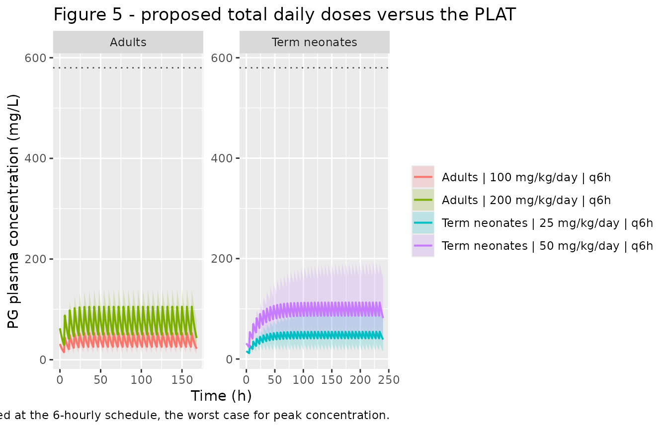
p95_max <- vpc |>
  group_by(arm, time) |>
  summarise(Q95 = quantile(Cc, 0.95), .groups = "drop") |>
  group_by(arm) |>
  summarise(`95th percentile peak (mg/L)` = round(max(Q95), 1), .groups = "drop") |>
  mutate(`Below PLAT?` = if_else(`95th percentile peak (mg/L)` < PLAT, "yes", "no"))
knitr::kable(p95_max,
             caption = paste("Upper (95th percentile) peak concentration for each proposed",
"regimen against the 580 mg/L PLAT."))| arm | 95th percentile peak (mg/L) | Below PLAT? |
|---|---|---|
| Adults | 100 mg/kg/day | q6h | 69.7 | yes |
| Adults | 200 mg/kg/day | q6h | 140.6 | yes |
| Term neonates | 25 mg/kg/day | q6h | 100.3 | yes |
| Term neonates | 50 mg/kg/day | q6h | 192.1 | yes |
Every proposed regimen stays below the PLAT across the upper 95th percentile of the simulated population, reproducing the paper’s central dosing recommendation.
Assumptions and deviations
-
The packaged models are compartmental reductions of a
platform PBPK model, not PBPK models. The source model’s
per-organ partition coefficients, organ volumes and blood flows are
Simcyp database outputs and are not published. The reduction keeps
everything the paper does publish (Vss,
ka,fa, the in-vitro Michaelis constant, renal clearance, the ADH ontogeny function) and collapses the whole-body distribution into a single central compartment sized by the published Vss. PG is a small, neutral, highly water-soluble molecule with a plasma unbound fraction of 0.99 and a Vss close to total body water, so distribution is effectively instantaneous and the one-compartment reduction is well justified. Its adequacy is demonstrated rather than assumed by the half-life, clearance-split, saturation, and PLAT checks above. -
vmaxis back-solved, not transcribed. Table 2’s in-vitro 1.57 nmole/min/mg of cytosolic protein cannot be scaled to a whole-body rate without the liver weight and the cytosolic-protein-per-gram-liver scalar, which are platform system parameters absent from the paper.vmaxis instead fixed by the identityvmax = CL_hepatic * kmusing Table 3’s predicted hepatic clearances. No parameter was tuned against a validation target. The paper publishes no liver weight or cytosolic-protein scalar for either population, so the twovmaxvalues are not cross-checked against an independent in-vitro-to-in-vivo scaling here; what is checked is that the resulting clearances, half-lives and saturation behaviour all reproduce the paper’s published values. - Reference body weights are not published. 70 kg (adult) and 3.5 kg (term neonate) are used. Because Vss is parameterised per kilogram and the paper’s doses are in mg/kg, the initial concentration after a dose is independent of this choice; only the half-life and accumulation depend on it, and both reference weights are corroborated by the resulting half-lives falling inside the paper’s published ranges (2-5 h and 10-31 h respectively).
- Clearance is not weight-scaled. The paper reports Vss per kilogram but hepatic and renal clearance as absolute L/h for each simulated population, and publishes no allometric exponent for either arm. No weight scaling was invented for the clearance terms, so the models should be used near their reference weights.
-
Equation (2) is documented but not implemented. The
paper derives neonatal renal function from
GFR (mL/min) = -19.8 + 89.04*BSA - 7.16*BSA^2. That polynomial parameterises the population glomerular filtration rate rather than PG renal clearance itself – PG is extensively reabsorbed, so its renal clearance is well below GFR in both populations – and it is numerically unstable at neonatal body surface areas, returning small negative values near a term neonate’s BSA. The published renal clearances of Table 3 are used directly instead. -
Variability terms are virtual-population output dispersions,
not estimated random effects. Table 3’s %CVs describe the
spread of predicted clearance across the 200-subject Simcyp populations,
driven by the platform’s physiological variability. They are encoded as
fixed etas on
vmaxandcl_renaland are labelled as such in both model files. No %CV is reported for the volume of distribution, sovccarries no eta. -
No residual error is available. The source is a
simulation study with no fitted residual-error model, so
propSdis fixed at 0. The models are intended for simulation, not for estimation against observed data as supplied. - The supplement was not available when this model was built. Section S1 (model development detail), Figures S1-S5 and Tables S1-S4 could not be consulted. No parameter used above comes from the supplement – every value is from Table 1, Table 2, Table 3, Equation (1) or the Results text – but the supplement’s Table S2 holds additional predicted-versus-observed PK parameters that would have supplied further validation targets.
- Saturation thresholds are compared structurally, not by the paper’s detection rule. The paper flagged saturation as a 1% departure from a linear-phase regression fitted across a 200-subject virtual population in GraphPad. That detection rule cannot be reproduced from a typical-value profile and is much more sensitive than the doses it reports, so the comparison above instead uses two zero-free-parameter structural consequences of the reduction: the constant ratio of threshold concentration to Michaelis constant across populations, and the accumulation-driven fall of the threshold with dosing frequency.
- Term neonates only. Equation (1) is continuous in age, so the neonatal model’s ADH ontogeny extends across childhood; its distribution and renal parameters, however, are term-neonate values. The paper is explicit that clinically observed PG concentration-time data are unavailable for older pediatric age groups, so the model should be used at neonatal ages.