Mosunetuzumab, preclinical and human-projected PK (Ferl 2018)
Source:vignettes/articles/Ferl_2018_mosunetuzumab.Rmd
Ferl_2018_mosunetuzumab.RmdModel and source
- Citation: Ferl GZ, Reyes A, Sun LL, Cheu M, Oldendorp A, Ramanujan S, Stefanich EG. A Preclinical Population Pharmacokinetic Model for Anti-CD20/CD3 T-Cell-Dependent Bispecific Antibodies. Clin Transl Sci. 2018;11(3):296-304. doi:10.1111/cts.12535
- Article: https://doi.org/10.1111/cts.12535 (open access, PMC5944627)
- Supplement: Supporting Information
CTS-11-296-s001.pdf(Tables S1-S4, Figures S1-S8), via the journal page or Europe PMC.
Ferl 2018 analysed the PK of BTCT4465A, the Genentech development code for the anti-CD20/CD3 T-cell-dependent bispecific antibody mosunetuzumab. The paper predates the INN and never uses it. The paper contributes three model files:
| Model file | Source | Content |
|---|---|---|
Ferl_2018_mosunetuzumab_cyno |
Table 2 | Cynomolgus-monkey base Model VI (no covariates) |
Ferl_2018_mosunetuzumab_cyno_covariates |
Table S3, Table S2 | Cynomolgus-monkey final model with covariates |
Ferl_2018_mosunetuzumab_human |
Table S3, Table 3, Eq. (8) | Typical-value allometric projection to a 70 kg human (Figure 4) |
All three share the structure of Eqs. (1)-(3) and Figure 1: a two-compartment model with first-order SC absorption and three elimination terms acting on the central compartment,
where t is the time since the first dose. In the model
files CL1 is cl_exp_inf, CL2_0 is
cl_exp_component, lambda2 is
cl_exp_kdes, Vmax_0 is vmax and
lambda1 is vmax_exp_kdes.
Population
Seven NHP safety / PK studies in healthy, purpose-bred, treatment-naive cynomolgus monkeys of Chinese origin (Charles River Laboratories, Reno, NV). The single-dose studies gave a slow IV bolus of 0.001-1 mg/kg to 3-4 animals per group. The repeat-dose studies gave 0.01-1 mg/kg once weekly for four doses, as a slow IV bolus or a 1-h infusion, or 1 mg/kg SC, to 3-8 animals per group. The median body weight was 3.12 kg and the median baseline CD4+ count was 2134 cells/uL (Table S3 caption). Two cohorts received CHO-derived material, most of it in one study with n = 44, and the rest received E. coli-derived material. The paper does not report the total number of animals. ADA-positive samples were excluded (Methods).
A naive-pooled fit to human CD20 / human CD3 double-transgenic mice (Figure 2a) is not packaged. Its V1, V2 and CLd are not reported (see Assumptions and deviations).
Source trace
Values per kg in Tables 2 and S3 were normalised by the 3.12 kg median body weight in a post hoc step (table footnotes), so the cyno files multiply them back by 3.12 kg. The human file scales the Table S3 values by Eq. (8).
| Parameter (paper) | Model name | Base (Table 2) | Covariates (Table S3) | Human (70 kg) |
|---|---|---|---|---|
| Ka (1/day) | lka |
1.33 | 1.26 | not projected |
| Z, F = 1/(1+exp(-Z)) | logitfdepot |
1.66 | 1.58 | not projected |
| CL1 (mL/day/kg) | lcl_exp_inf |
7.05 | 6.95 | 6.95 x 3.12 x (70/3.12)^0.85 |
| CL2_0 (mL/day/kg) | lcl_exp_component |
63.8 | 855 (E. coli) / 120 (CHO) | 18.0 mL/day (Table 3, rituximab NHL) |
| lambda2 (1/day) | lcl_exp_kdes |
10.1 | 35.2 | 0.023 (Table 3, rituximab NHL) |
| CLd (mL/day/kg) | lq |
31.3 | 34.3 (E. coli) / 61.8 (CHO) | 34.3 x 3.12 x (70/3.12)^0.85 |
| V1 (mL/kg) | lvc |
44.4 | 43.6 (E. coli) / 108 (CHO) | 43.6 x 70 |
| V2 (mL/kg) | lvp |
47.3 | 40.4 | 40.4 x 70 |
| Vmax_0 (ug/day) | lvmax |
1280 | 1760 | 1760 x 70/3.12 |
| lambda1 (1/day) | lvmax_exp_kdes |
0.144 | 0.167 | 0.167 (NHP value) |
| KM (ug/mL) | lkm |
19.6 | 31.1 | 31.1 (not scaled) |
| theta CD4 on CL1 | e_cd4_abs_cl_exp_inf |
- | 0.000314 | - |
| theta CD4 on lambda1 | e_cd4_abs_vmax_exp_kdes |
- | 0.000371 | - |
| theta BW on lambda2 | e_wt_cl_exp_kdes |
- | -0.562 | - |
| IIV (%CV): CL2_0, Vmax_0, CL1, CLd, V1, V2 | eta... |
82, 41, 25, 69, 41, 31 (diagonal) | Table S2 full block | none |
| Residual error | propSd |
proportional, not reported | proportional, not reported | none |
Equations: Eqs. (1)-(3) for the ODEs, Eq. (4) for log-normal IIV, Eq.
(5) %CV = 100 * sqrt(exp(omega^2) - 1), Eq. (6) for the
linear covariate form
p = p_pop * exp(eta) * (1 + theta * (cov - median)), and
Eq. (8) for the allometric scaling. The scaling exponents come from
Methods “Allometric scaling”.
Cynomolgus monkey base model: Figure 2b
Figure 2b compares a VPC of Model VI with the 1 mg/kg once-weekly x 4 IV cohort. A slow IV push is a bolus, as in the paper (Methods).
mod_cyno <- readModelDb("Ferl_2018_mosunetuzumab_cyno")
wt_cyno <- 3.12
n_sub <- 200

ev_cyno <- et(amt = 1 * wt_cyno, cmt = "central", ii = 7, addl = 3) |>
  et(c(seq(0, 1, by = 0.05), seq(1.25, 77, by = 0.25)), cmt = "central") |>
  et(id = seq_len(n_sub))

rxode2::rxSetSeed(20180119)
sim_cyno <- rxSolve(mod_cyno, ev_cyno, returnType = "data.frame")
#> ℹ parameter labels from comments will be replaced by 'label()'

vpc_cyno <- sim_cyno |>
  filter(Cc > 0) |>
  group_by(time) |>
  summarise(
    med = median(Cc),
    lo = quantile(Cc, 0.05),
    hi = quantile(Cc, 0.95),
    .groups = "drop"
  )

ggplot(vpc_cyno, aes(time, med)) +
  geom_ribbon(aes(ymin = lo, ymax = hi), fill = "steelblue", alpha = 0.3) +
  geom_line(colour = "steelblue4") +
  geom_vline(xintercept = c(0, 7, 14, 21), linetype = "dotted") +
  scale_y_log10() +
  labs(
    x = "Time (day)", y = "Mosunetuzumab (ug/mL)",
    caption = "Replicates Figure 2b of Ferl 2018: median and 5-95% interval, 1 mg/kg IV weekly x 4."
  )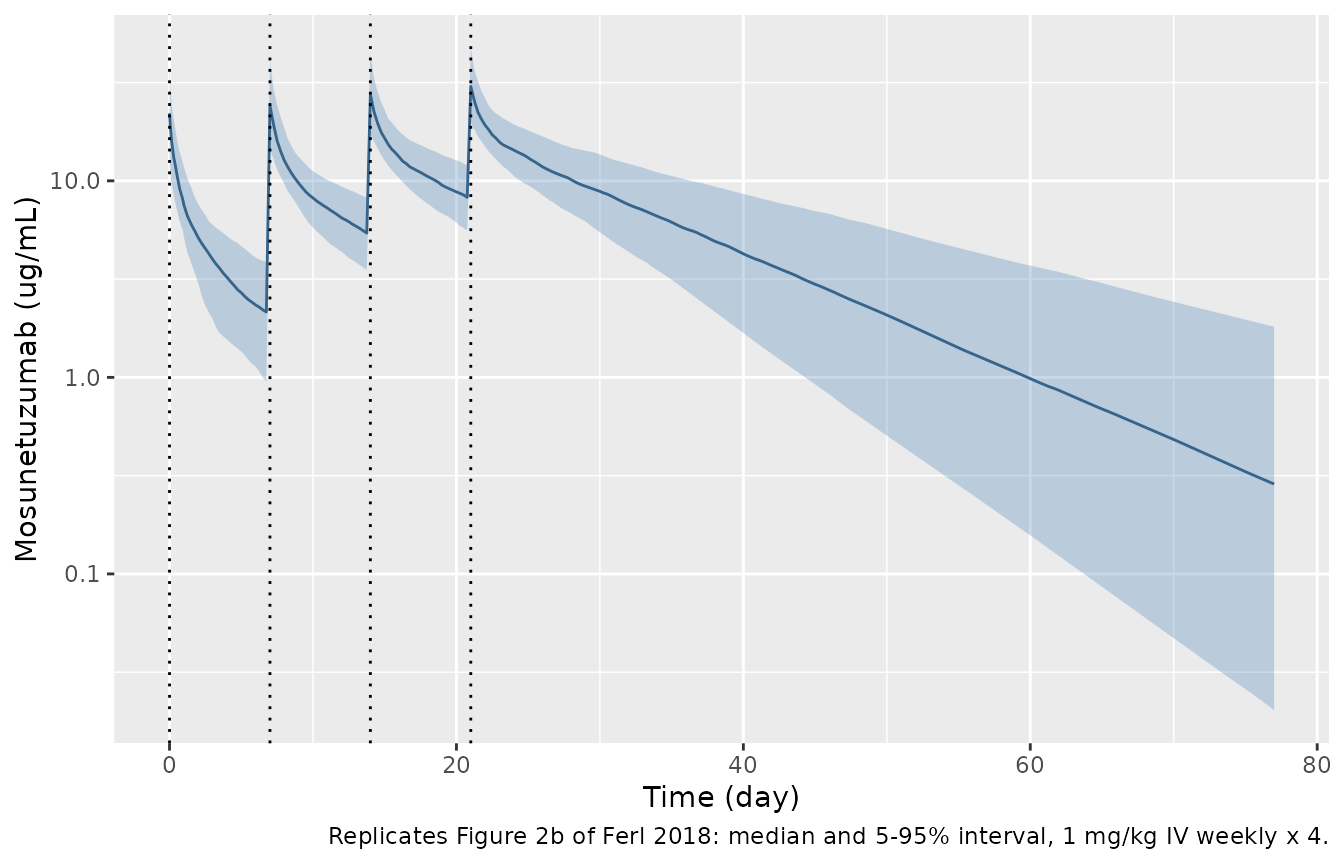
The simulated median starts at about 22 ug/mL (1 mg/kg over V1 = 44.4 mL/kg) and falls more steeply after the first dose than after the fourth. That is the time-varying clearance the paper reports for days 0-7 versus days 21-28.
Fractional elimination rates: Figure 3
Figure 3 splits the fractional elimination rate (1/day) into the
constant linear term CL1/V1, the decaying linear term
CL2(t)/V1 and the decaying nonlinear term
(Vmax(t)/V1)/(C + KM). These are typical-value curves for
weekly x 4 IV dosing across the NHP dose range.
mod_cyno_typ <- rxode2::zeroRe(mod_cyno)
#> ℹ parameter labels from comments will be replaced by 'label()'
frac <- bind_rows(lapply(c(0.01, 0.1, 1), function(dose_mgkg) {
  ev <- et(amt = dose_mgkg * wt_cyno, cmt = "central", ii = 7, addl = 3) |>
    et(seq(0, 35, by = 0.05), cmt = "central")
  rxSolve(mod_cyno_typ, ev, returnType = "data.frame") |>
    mutate(
      dose = paste(dose_mgkg, "mg/kg"),
      `Constant linear` = cl_exp_inf / vc,
      `Time-varying linear` = cl_exp_component * exp(-cl_exp_kdes * time) / vc,
      `Time-varying nonlinear` = vmax_t / vc / (Cc + km)
    )
})) |>
  select(time, dose, `Constant linear`, `Time-varying linear`, `Time-varying nonlinear`) |>
  pivot_longer(-c(time, dose), names_to = "term", values_to = "rate")
#> ℹ omega/sigma items treated as zero: 'etalcl_exp_component', 'etalvmax', 'etalcl_exp_inf', 'etalq', 'etalvc', 'etalvp'
#> ℹ omega/sigma items treated as zero: 'etalcl_exp_component', 'etalvmax', 'etalcl_exp_inf', 'etalq', 'etalvc', 'etalvp'
#> ℹ omega/sigma items treated as zero: 'etalcl_exp_component', 'etalvmax', 'etalcl_exp_inf', 'etalq', 'etalvc', 'etalvp'

ggplot(frac, aes(time, rate, colour = dose)) +
  geom_line() +
  facet_wrap(~term, scales = "free_y") +
  labs(
    x = "Time (day)", y = "Fractional elimination rate (1/day)",
    caption = "Replicates Figure 3a-b of Ferl 2018 (typical values, weekly x 4 IV)."
  )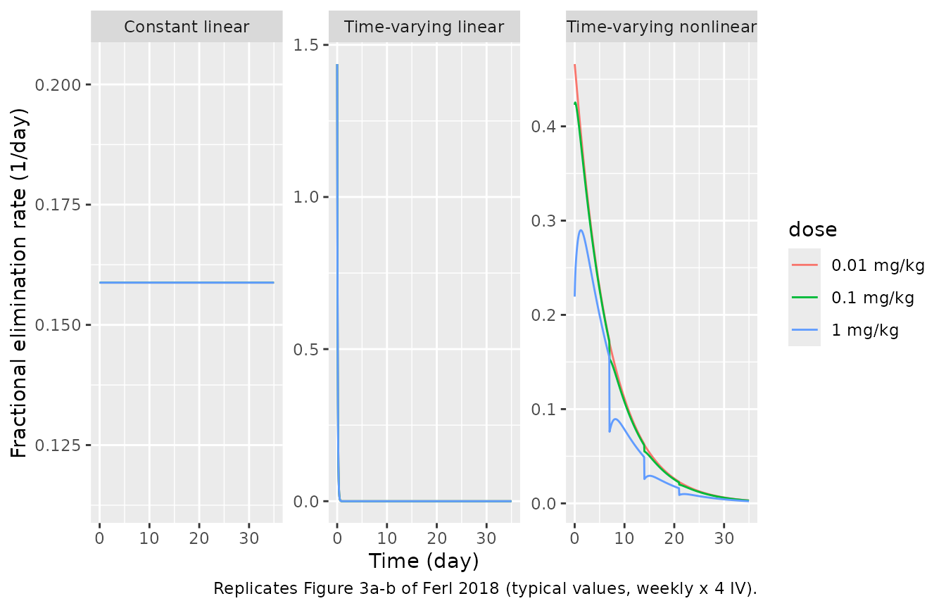
The linear time-varying term halves every
log(2)/10.1 = 0.069 day (1.6 h), and the nonlinear term’s
Vmax halves every log(2)/0.144 = 4.8 days, matching the
half-lives quoted in the abstract. The nonlinear term rises as the
concentration falls below KM, so it peaks later at higher doses. At 1
mg/kg the typical curve peaks about 1.2 days after the first dose,
against the “2 days postinjection” in the Results.
Cynomolgus monkey model with covariates (Table S3)
The final model adds the cell-line source on V1, CLd and CL2_0, the baseline CD4+ count on CL1 and lambda1, and body weight on lambda2. The typical profiles below show each effect for 1 mg/kg weekly x 4 IV in a 3.12 kg animal.
mod_cov <- rxode2::zeroRe(readModelDb("Ferl_2018_mosunetuzumab_cyno_covariates"))
#> ℹ parameter labels from comments will be replaced by 'label()'
scen <- tribble(
  ~scenario, ~FORM_MOSU_CHO, ~CD4_ABS, ~WT,
  "E. coli, CD4 2134, 3.12 kg (reference)", 0, 2134, 3.12,
  "CHO, CD4 2134, 3.12 kg", 1, 2134, 3.12,
  "E. coli, CD4 1000, 3.12 kg", 0, 1000, 3.12,
  "E. coli, CD4 5000, 3.12 kg", 0, 5000, 3.12,
  "E. coli, CD4 2134, 2.5 kg", 0, 2134, 2.5,
  "E. coli, CD4 2134, 4.5 kg", 0, 2134, 4.5
) |>
  mutate(id = row_number())

ev_cov <- et(amt = 1 * wt_cyno, cmt = "central", ii = 7, addl = 3) |>
  et(c(seq(0, 1, by = 0.02), seq(1.1, 42, by = 0.1)), cmt = "central") |>
  et(id = scen$id) |>
  as.data.frame() |>
  left_join(scen, by = "id")

sim_cov <- rxSolve(mod_cov, ev_cov, returnType = "data.frame", keep = "scenario")
#> ℹ omega/sigma items treated as zero: 'etalcl_exp_component', 'etalvmax', 'etalcl_exp_inf', 'etalq', 'etalvc', 'etalvp'
#> Warning: multi-subject simulation without without 'omega'

ggplot(sim_cov, aes(time, Cc, colour = scenario)) +
  geom_line() +
  scale_y_log10() +
  labs(x = "Time (day)", y = "Mosunetuzumab (ug/mL)", colour = NULL) +
  theme(legend.position = "bottom", legend.direction = "vertical")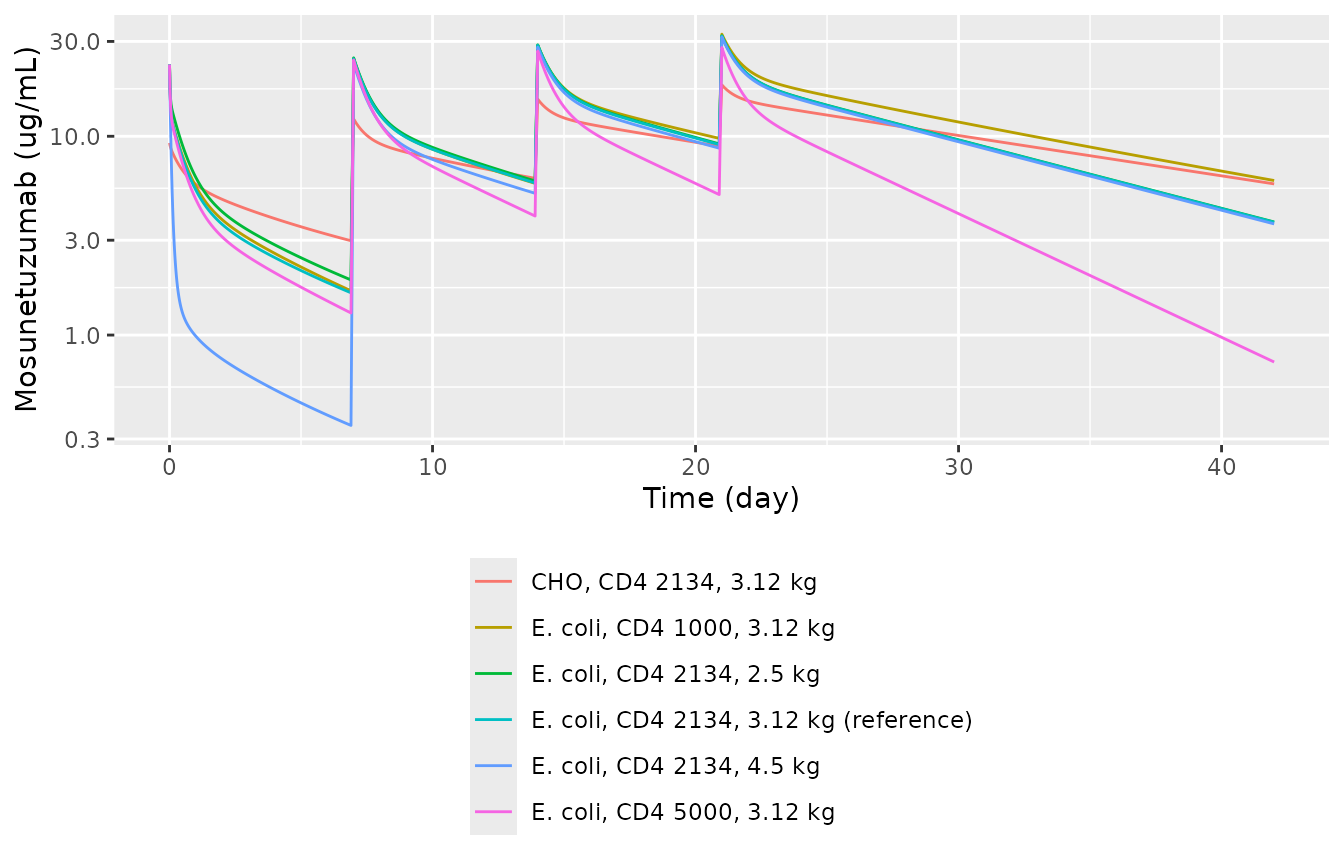
CHO-derived material has a larger V1 (108 vs 43.6 mL/kg), so its first peak is lower, and a much smaller initial decaying clearance (120 vs 855 mL/day/kg). A higher baseline CD4+ count raises CL1 and speeds the decay of the saturable pathway, the direction shown in Figure S8. The body-weight effect on lambda2 is a linear slope of -0.562 per kg, so lambda2 reaches zero at 4.90 kg.
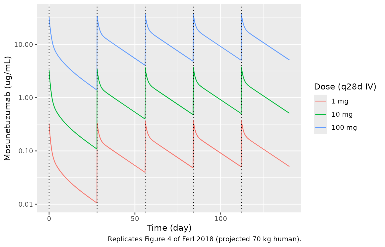
Human projection: Figure 4
Figure 4 projects mean PK in a 70 kg human for 1, 10 and 100 mg flat IV doses every 28 days, and its inset tabulates Cmax, Cmin and AUC for cycles 1 and 5. Cycle 1 is computed from a single dose (identical to the multiple-dose profile up to day 28), and cycle 5 from the fifth dose at day 112.
mod_h <- readModelDb("Ferl_2018_mosunetuzumab_human")
doses <- c(1, 10, 100)
grid_c1 <- c(seq(0, 1, by = 0.01), seq(1.05, 28, by = 0.05))

sim_h <- bind_rows(lapply(seq_along(doses), function(i) {
  d <- doses[i]
  ev_md <- et(amt = d, cmt = "central", ii = 28, addl = 4) |>
    et(c(grid_c1, 112 + grid_c1), cmt = "central")
  ev_sd <- et(amt = d, cmt = "central") |>
    et(grid_c1, cmt = "central")
  bind_rows(
    rxSolve(mod_h, ev_sd, returnType = "data.frame") |> mutate(cycle = "1"),
    rxSolve(mod_h, ev_md, returnType = "data.frame") |>
      filter(time >= 112) |>
      mutate(cycle = "5")
  ) |>
    mutate(id = i, treatment = paste(d, "mg"))
}))

prof_h <- bind_rows(lapply(seq_along(doses), function(i) {
  ev <- et(amt = doses[i], cmt = "central", ii = 28, addl = 4) |>
    et(seq(0, 140, by = 0.1), cmt = "central")
  rxSolve(mod_h, ev, returnType = "data.frame") |>
    mutate(treatment = paste(doses[i], "mg"))
}))

ggplot(prof_h, aes(time, Cc, colour = treatment)) +
  geom_line() +
  scale_y_log10() +
  geom_vline(xintercept = seq(0, 112, by = 28), linetype = "dotted") +
  labs(
    x = "Time (day)", y = "Mosunetuzumab (ug/mL)", colour = "Dose (q28d IV)",
    caption = "Replicates Figure 4 of Ferl 2018 (projected 70 kg human)."
  )
conc_h <- sim_h |>
  filter(!is.na(Cc)) |>
  select(id, treatment, cycle, time, Cc)
dose_h <- conc_h |>
  distinct(id, treatment, cycle) |>
  mutate(time = ifelse(cycle == "1", 0, 112), amt = as.numeric(sub(" mg", "", treatment)))

o_conc <- PKNCAconc(conc_h, Cc ~ time | treatment + cycle / id)
o_dose <- PKNCAdose(dose_h, amt ~ time | treatment + cycle + id)
intervals_h <- tidyr::crossing(treatment = unique(conc_h$treatment), cycle = c("1", "5")) |>
  mutate(
    start = ifelse(cycle == "1", 0, 112),
    end = start + 28,
    cmax = TRUE, cmin = TRUE, auclast = TRUE
  )
nca_h <- pk.nca(PKNCAdata(o_conc, o_dose, intervals = intervals_h))

# Figure 4 inset (Cmax and Cmin in ug/mL, AUC in ug/mL*day)
ref_h <- tribble(
  ~treatment, ~cycle, ~cmax, ~cmin, ~auclast,
  "1 mg", "1", 0.32, 0.01, 1,
  "10 mg", "1", 3.2, 0.11, 10.6,
  "100 mg", "1", 33, 1.4, 128,
  "1 mg", "5", 0.38, 0.051, 3.2,
  "10 mg", "5", 3.8, 0.51, 32,
  "100 mg", "5", 38, 5.1, 325
)

cmp_h <- ncaComparisonTable(
  as.data.frame(nca_h$result),
  ref_h,
  by = c("treatment", "cycle"),
  units = c(cmax = "ug/mL", cmin = "ug/mL", auclast = "ug*day/mL")
)
knitr::kable(cmp_h, caption = "Simulated vs Figure 4 inset of Ferl 2018 (70 kg human, q28d IV).")| NCA parameter | treatment | cycle | Reference | Simulated | % diff |
|---|---|---|---|---|---|
| Cmax (ug/mL) | 1 mg | 1 | 0.32 | 0.328 | +2.4% |
| Cmax (ug/mL) | 1 mg | 5 | 0.38 | 0.378 | -0.6% |
| Cmax (ug/mL) | 10 mg | 1 | 3.2 | 3.28 | +2.4% |
| Cmax (ug/mL) | 10 mg | 5 | 3.8 | 3.78 | -0.6% |
| Cmax (ug/mL) | 100 mg | 1 | 33 | 32.8 | -0.7% |
| Cmax (ug/mL) | 100 mg | 5 | 38 | 37.8 | -0.6% |
| Cmin (ug/mL) | 1 mg | 1 | 0.01 | 0.0105 | +4.6% |
| Cmin (ug/mL) | 1 mg | 5 | 0.051 | 0.0509 | -0.2% |
| Cmin (ug/mL) | 10 mg | 1 | 0.11 | 0.108 | -1.9% |
| Cmin (ug/mL) | 10 mg | 5 | 0.51 | 0.509 | -0.2% |
| Cmin (ug/mL) | 100 mg | 1 | 1.4 | 1.38 | -1.3% |
| Cmin (ug/mL) | 100 mg | 5 | 5.1 | 5.09 | -0.2% |
| AUClast (ug*day/mL) | 1 mg | 1 | 1 | 1.03 | +3.3% |
| AUClast (ug*day/mL) | 1 mg | 5 | 3.2 | 3.25 | +1.5% |
| AUClast (ug*day/mL) | 10 mg | 1 | 10.6 | 10.6 | -0.0% |
| AUClast (ug*day/mL) | 10 mg | 5 | 32 | 32.5 | +1.6% |
| AUClast (ug*day/mL) | 100 mg | 1 | 128 | 128 | +0.2% |
| AUClast (ug*day/mL) | 100 mg | 5 | 325 | 325 | +0.0% |
sim_wide <- as.data.frame(nca_h$result) |>
  select(treatment, cycle, PPTESTCD, PPORRES) |>
  pivot_wider(names_from = PPTESTCD, values_from = PPORRES) |>
  left_join(ref_h, by = c("treatment", "cycle"), suffix = c("_sim", "_ref"))
# Deterministic typical-value solve against a printed table: every Cmin and AUC
# reproduces the inset to within its printed rounding plus a few percent.
stopifnot(
  all(abs(sim_wide$auclast_sim / sim_wide$auclast_ref - 1) < 0.05),
  all(abs(sim_wide$cmin_sim / sim_wide$cmin_ref - 1) < 0.10),
  all(abs(sim_wide$cmax_sim / sim_wide$cmax_ref - 1) < 0.05)
)
Cmin and AUC reproduce the inset at all three doses and both cycles,
as does steady-state Cmax. Cycle-1 Cmax is dose / V1, which
gives 0.328 and 3.28 ug/mL against the printed 0.32 and 3.2. The 2.5%
gap is within the uncertainty of how the paper read Cmax off its
simulation grid.
Assumptions and deviations
- Drug name. The paper calls the molecule only BTCT4465A. BTCT4465A is the Genentech development code for mosunetuzumab (RG7828; ClinicalTrials.gov NCT02500407), and the file stems use the INN per the library’s naming policy.
- Per-kg normalisation undone. CL1, CL2_0, CLd, V1 and V2 were divided by the 3.12 kg median body weight after fitting (Table 2 and Table S3 footnotes), so the cyno files carry absolute values for a 3.12 kg animal. Vmax_0 was not normalised. Table 2 prints its units as ug/mL, but the Results text (“1,280 ug/day”) and Table S3 give ug/day.
-
Table S2 belongs to the covariate model. Table S2
is captioned as the base Model VI variance-covariance matrix. Through
Eq. (5), however, its diagonal gives %CVs of 20, 40, 59, 39, 39 and 44
for CL1, CL2_0, CLd, V1, V2 and Vmax_0. Those are the Table S3
covariate-model %CVs (printed 20, 40, 59, 39, 38, 44), not the Table 2
base-model %CVs (25, 82, 69, 41, 31, 41). The Results text (“20, 50, 15,
and 5% lower … compared with the base model”) confirms both tables’
%CVs. The covariate model therefore carries the full Table S2 block. The
base model carries the Table 2 variances,
omega^2 = log(1 + CV^2), with no covariances, because no base-model covariances are reported. - Table S2 nudged to positive definite. Rounded to two decimals, the matrix has a smallest eigenvalue of -0.00095 (the CL2_0-V1 correlation is -0.97). The off-diagonals are scaled by 0.99, and the variances are unchanged.
-
Residual error. The supplement (section B.9) states
a proportional error model but reports no magnitude, so
propSdis held at zero. - Human projection uses Table S3, and CL2_0 = 18 mL/day. The Figure 4 caption reads “the final model with covariates scaled from NHP (Table 2)”, and the Results text says “using the final model with covariates”. The inset decides between them. With the Table S3 values (E. coli reference, median CD4+) and CL2_0 = 18.0 mL/day for the whole body, every Cmin and AUC and the steady-state Cmax reproduce. With the Table 2 values, cycle-1 AUCs are 7% to 15% low. Table 3 prints the rituximab NHL CL2_0 as 18.0 mL/day/kg, but applying it per kg (18.0 x 70 = 1.26 L/day) puts the cycle-1 AUCs 2.4-fold below the inset and the cycle-5 AUCs 25% below it. The packaged human file follows the reading that reproduces the published projection.
- Internal inconsistencies in the source. The Results text gives steady-state Cmax as 0.37, 3.7 and 37 ug/mL. The inset prints 0.38, 3.8 and 38, and the model gives 0.378, 3.78 and 37.8. The text’s AUC accumulation of “268%, 253%, and 169%” matches no reading of the inset: the inset ratios are 3.20, 3.02 and 2.54.
- Human file scope. The human file is a typical-value projection: no between-subject variability and no SC absorption were projected. The CD4+ and body-weight effects are at their NHP medians (the CD4+ effect only acts through lambda1 = 0.167 1/day). The authors caution that KM, Vmax_0, CL2_0, lambda1 and lambda2 should not be extrapolated to humans without clinical data (Discussion).
- Body weight on lambda2. The linear slope makes lambda2 zero at 4.90 kg and negative above it, which is an exponentially growing clearance. The cohort’s weight range is not reported. Do not use the covariate model for heavier animals.
- Murine sub-model not packaged. Figure 2a gives only CL1 = 16 mL/day/kg, KM = 0.015 ug/mL and a constant Vmax = 12 ug/day for the naive-pooled mouse fit. V1, V2 and CLd appear nowhere in the paper or supplement, so the model cannot be written without inventing them.
-
Time origin.
tin CL2(t) and Vmax(t) is the time since the first dose and does not reset at later doses, matching Figure 3, where the decaying terms continue across the dosing interval.