Theophylline PK and neonatal weight change (Rohleff 2025)
Source:vignettes/articles/Rohleff_2025_theophylline_neonatalWeight.Rmd
Rohleff_2025_theophylline_neonatalWeight.RmdModel and source
Rohleff 2025 introduces a variational-autoencoder (VAE) estimator for nonlinear mixed-effects models that estimates the population parameters and selects covariates in a single run. The paper demonstrates it on two real datasets, and each fitted model is packaged here:
Rohleff_2025_theophylline– one-compartment oral PK of theophylline in 12 subjects (Section 3.1, Table 1).Rohleff_2025_neonatalWeight– body-weight change over the first week of life in 2425 neonates (Section 3.2, Supporting Information Table S3).Citation: Rohleff J, Bachmann F, Nahum U, Bram D, Steffens B, Pfister M, Koch G, Schropp J. Redefining Parameter Estimation and Covariate Selection via Variational Autoencoders: One Run Is All You Need. CPT Pharmacometrics Syst Pharmacol. 2025;14(8):2232-2243. doi:10.1002/psp4.70129.
Article: https://doi.org/10.1002/psp4.70129 (open access, PMC12706427)
Code: https://github.com/janrohleff/vae_nlme (the authors’ Python implementation)
Both models use the estimates from the paper’s own method (the VAE column). The paper also reports the same models fitted with SAEM-based methods (COSSAC, SAMBA and SCM for theophylline, SAEM for the neonates); those are used below as comparisons, not as alternative model files.
Population
Theophylline. Twelve subjects each received a single
oral theophylline dose at time zero, with plasma concentrations measured
over about 24 h and baseline weight and sex recorded (Section 3.1). This
is the classic dataset distributed with NONMEM and with R as
datasets::Theoph (Pinheiro and Bates 2000, the paper’s
reference 18). Weights range from 54.6 to 86.4 kg (mean 69.6 kg), 5 of
12 subjects are female, and the doses are 3.10-5.86 mg/kg, about 320 mg
in total for 11 subjects and 268 mg for one.
Neonates. 2425 neonates had their body weight measured repeatedly over the first 7 days of life (Section 3.2), with sex, mode of delivery, gestational age, maternal age and parity as candidate covariates. The cohort is that of Wilbaux et al. (J Pediatr 2016; Clin Nutr 2019), both of which describe term neonates. The paper gives no demographic table and the data are not public.
str(readModelDb("Rohleff_2025_theophylline")()$population, give.attr = FALSE)
#> List of 9
#>  $ species       : chr "human"
#>  $ n_subjects    : int 12
#>  $ n_studies     : int 1
#>  $ weight_range  : chr "54.6-86.4 kg (mean 69.6 kg; authors' deposited dataset)"
#>  $ sex_female_pct: num 41.7
#>  $ disease_state : chr "Not stated in the paper ('N = 12 patients'); the dataset is the classic theophylline study distributed with NON"| __truncated__
#>  $ dose_range    : chr "Single oral theophylline loading dose at t = 0; 267.8-320.7 mg total (3.10-5.86 mg/kg) in the deposited dataset."
#>  $ n_observations: int 120
#>  $ notes         : chr "Section 3.1 'Data': plasma theophylline concentrations from 12 subjects after a single oral dose at t = 0, with"| __truncated__
str(readModelDb("Rohleff_2025_neonatalWeight")()$population, give.attr = FALSE)
#> List of 7
#>  $ species      : chr "human"
#>  $ n_subjects   : int 2425
#>  $ n_studies    : int 1
#>  $ age_range    : chr "Birth to 7 days postnatal age"
#>  $ disease_state: chr "Neonates followed over the first week of life (the cohort of Wilbaux et al., J Pediatr 2016 and Clin Nutr 2019,"| __truncated__
#>  $ dose_range   : chr "n/a (no drug)"
#>  $ notes        : chr "Section 3.2 'Data': repeated body weights from 2425 neonates over the first 7 days of life, with sex, mode of d"| __truncated__
Source trace
| Model | Parameter / equation | Value | Source location |
|---|---|---|---|
| theophylline | lka |
log(1.63) 1/h | Table 1, VAE, ka,pop
|
| theophylline | lkel |
log(0.086) 1/h | Table 1, VAE, ke,pop
|
| theophylline | lvc |
log(31.97) L | Table 1, VAE, Vpop
|
| theophylline | e_wt_ka |
2.55 | Table 1, VAE, beta_ka,w
|
| theophylline | e_wt_vc |
0.57 | Table 1, VAE, beta_V,w
|
| theophylline | etalka |
0.2809 (= 0.53^2) | Table 1, VAE, omega_ka (SD) |
| theophylline | etalkel |
0.0225 (= 0.15^2) | Table 1, VAE, omega_ke (SD) |
| theophylline | etalvc |
0.0169 (= 0.13^2) | Table 1, VAE, omega_V (SD) |
| theophylline | addSd |
0.71 mg/L | Table 1, VAE, error model a
|
| theophylline | weight reference 69.583 kg | mean of the 12 weights | Section 3.1 (w_pop = mean weight); value computed from
the authors’ deposited dataset |
| theophylline |
d/dt(depot), d/dt(central),
Cc = central / vc
|
Equation 14 and the line after it | |
| theophylline | log-normal individual parameters with log(w / w_pop)
covariate |
Section 3.1, ‘Model Description’ | |
| neonatal weight |
lrbase (W0) |
log(3383.2) g | Table S3, VAE, W0,pop
|
| neonatal weight | lkin |
log(106.8) g/day | Table S3, VAE, kin,pop
|
| neonatal weight |
lkin_t50 (Tlag) |
log(1.56) day | Table S3, VAE, Tlag,pop
|
| neonatal weight | lkout |
log(0.072) 1/day | Table S3, VAE, kout,pop
|
| neonatal weight |
lkout_t50 (T50) |
log(1.18) day | Table S3, VAE, T50,pop
|
| neonatal weight | etalrbase |
0.0196 (= 0.14^2) | Table S3, VAE, omega_W0 (SD) |
| neonatal weight | etalkin |
0.0529 (= 0.23^2) | Table S3, VAE, omega_kin (SD) |
| neonatal weight | etalkin_t50 |
0.0144 (= 0.12^2) | Table S3, VAE, omega_Tlag (SD) |
| neonatal weight | etalkout |
0.0100 (= 0.10^2) | Table S3, VAE, omega_kout (SD) |
| neonatal weight | etalkout_t50 |
0.0576 (= 0.24^2) | Table S3, VAE, omega_T50 (SD) |
| neonatal weight | addSd |
33.0 g | Table S3, VAE, error model a
|
| neonatal weight |
d/dt(bw) = kprod - kelim * bw,
bw(0) = W0
|
Equation 15 | |
| neonatal weight |
kprod = kin / (1 + exp(-2 (t - Tlag))),
kelim = kout (1 - t / (T50 + t))
|
Equation 15 |
Both tables report omega as the standard deviation of a log-normal
random effect, so each ini() variance is the square of the
printed value. The residual error is a constant (additive) error model
in both cases (Equation 2).
Theophylline
Closed-form check
The authors’ decoder evaluates the analytic solution of Equation 14,
C(t) = D ka / (V (ka - ke)) (exp(-ke t) - exp(-ka t)). The
packaged ODE model is solved for a typical subject at the mean weight
and compared with it.
mod_theo <- readModelDb("Rohleff_2025_theophylline")
wt_ref <- 69.583
ev_typ <- dplyr::bind_rows(
  data.frame(id = 1L, time = 0, evid = 1L, amt = 320, cmt = "depot", WT = wt_ref),
  data.frame(
    id = 1L, time = seq(0.25, 24, by = 0.25), evid = 0L, amt = 0,
    cmt = "central", WT = wt_ref
  )
)
sim_typ <- rxode2::rxSolve(
  rxode2::zeroRe(mod_theo), events = ev_typ, rtol = 1e-10, atol = 1e-12
)
#> ℹ parameter labels from comments will be replaced by 'label()'
#> ℹ omega/sigma items treated as zero: 'etalka', 'etalkel', 'etalvc'
closed_form <- with(
  list(ka = 1.63, ke = 0.086, V = 31.97, D = 320),
  D * ka / (V * (ka - ke)) * (exp(-ke * sim_typ$time) - exp(-ka * sim_typ$time))
)
rel_err <- max(abs(sim_typ$Cc / closed_form - 1))
rel_err
#> [1] 2.890022e-11
# Measured ~3e-11 at these tolerances; the bound is far above that and far
# below any transcription error.
stopifnot(rel_err < 1e-7)
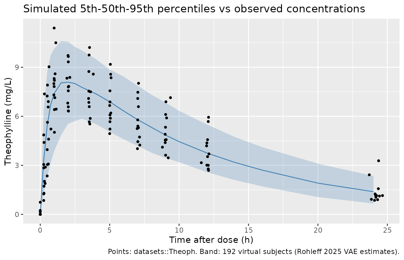
Virtual cohort and VPC against the observed data
The model was fitted to datasets::Theoph, so the
observed concentrations can be overlaid directly. Each of the 12
subjects (with their own weight and total dose) is replicated 16 times,
giving 192 virtual subjects.
theoph <- as.data.frame(datasets::Theoph) |>
  dplyr::mutate(
    id = as.integer(as.character(Subject)),
    amt = Dose * Wt
  )
subjects <- theoph |>
  dplyr::distinct(id, WT = Wt, amt)

n_rep <- 16L
grid <- c(0, 0.25, 0.5, 0.75, 1, 1.5, 2, 2.5, 3, 4, 5, 6, 7, 8, 9, 10, 12, 14, 16, 20, 24)
cohort <- tidyr::crossing(rep = seq_len(n_rep), subjects) |>
  dplyr::mutate(sim_id = (rep - 1L) * nrow(subjects) + id)
stopifnot(!anyDuplicated(cohort$sim_id), nrow(cohort) <= 200)

theo_events <- dplyr::bind_rows(
  cohort |>
    dplyr::transmute(id = sim_id, time = 0, evid = 1L, amt, cmt = "depot", WT),
  cohort |>
    dplyr::select(id = sim_id, WT) |>
    tidyr::crossing(time = grid) |>
    dplyr::mutate(evid = 0L, amt = 0, cmt = "central")
) |>
  dplyr::mutate(treatment = "Single oral dose") |>
  dplyr::arrange(id, time, dplyr::desc(evid))

rxode2::rxSetSeed(20251)
sim_theo <- rxode2::rxSolve(mod_theo, events = theo_events, keep = "treatment")
#> ℹ parameter labels from comments will be replaced by 'label()'
vpc <- as.data.frame(sim_theo) |>
  dplyr::group_by(time) |>
  dplyr::summarise(
    Q05 = quantile(Cc, 0.05), Q50 = median(Cc), Q95 = quantile(Cc, 0.95),
    .groups = "drop"
  )
ggplot(vpc, aes(time, Q50)) +
  geom_ribbon(aes(ymin = Q05, ymax = Q95), alpha = 0.25, fill = "steelblue") +
  geom_line(colour = "steelblue") +
  geom_point(data = theoph, aes(Time, conc), inherit.aes = FALSE, size = 1) +
  labs(
    x = "Time after dose (h)", y = "Theophylline (mg/L)",
    title = "Simulated 5th-50th-95th percentiles vs observed concentrations",
    caption = "Points: datasets::Theoph. Band: 192 virtual subjects (Rohleff 2025 VAE estimates)."
  )
PKNCA: simulated cohort vs the observed data
The paper reports no NCA, so the reference is NCA of the observed
datasets::Theoph profiles. The observed pre-dose samples
are set to zero, matching the data the authors fitted (which contain no
time-zero records).
nca_intervals <- data.frame(
  start = 0, end = Inf,
  cmax = TRUE, tmax = TRUE, auclast = TRUE, half.life = TRUE
)

sim_conc <- as.data.frame(sim_theo) |>
  dplyr::filter(!is.na(Cc)) |>
  dplyr::select(id, time, Cc, treatment)
sim_conc <- dplyr::bind_rows(
  sim_conc,
  sim_conc |> dplyr::distinct(id, treatment) |> dplyr::mutate(time = 0, Cc = 0)
) |>
  dplyr::distinct(id, treatment, time, .keep_all = TRUE) |>
  dplyr::arrange(id, time)
sim_dose <- theo_events |>
  dplyr::filter(evid == 1L) |>
  dplyr::select(id, time, amt, treatment)
nca_sim <- PKNCA::pk.nca(PKNCA::PKNCAdata(
  PKNCA::PKNCAconc(sim_conc, Cc ~ time | treatment + id),
  PKNCA::PKNCAdose(sim_dose, amt ~ time | treatment + id),
  intervals = nca_intervals
))

obs_conc <- theoph |>
  dplyr::transmute(id, time = Time, Cc = ifelse(Time == 0, 0, conc), treatment = "Single oral dose")
obs_dose <- subjects |>
  dplyr::transmute(id, time = 0, amt, treatment = "Single oral dose")
nca_obs <- PKNCA::pk.nca(PKNCA::PKNCAdata(
  PKNCA::PKNCAconc(obs_conc, Cc ~ time | treatment + id),
  PKNCA::PKNCAdose(obs_dose, amt ~ time | treatment + id),
  intervals = nca_intervals
))

obs_median <- as.data.frame(nca_obs) |>
  dplyr::group_by(treatment, PPTESTCD) |>
  dplyr::summarise(value = median(PPORRES, na.rm = TRUE), .groups = "drop") |>
  tidyr::pivot_wider(names_from = PPTESTCD, values_from = value)

cmp <- nlmixr2lib::ncaComparisonTable(
  simulated = nca_sim,
  reference = obs_median,
  by = "treatment",
  params = c("cmax", "tmax", "auclast", "half.life"),
  units = c(cmax = "mg/L", tmax = "h", auclast = "mg*h/L", half.life = "h"),
  tolerance_pct = 20
)
knitr::kable(
  cmp,
  caption = "Median NCA of the simulated cohort vs the observed datasets::Theoph profiles. * differs by >20%."
)| NCA parameter | treatment | Reference | Simulated | % diff |
|---|---|---|---|---|
| Cmax (mg/L) | Single oral dose | 8.46 | 8.37 | -1.2% |
| Tmax (h) | Single oral dose | 1.14 | 2 | +76.2%* |
| AUClast (mg*h/L) | Single oral dose | 92.3 | 100 | +8.5% |
| t½ (h) | Single oral dose | 7.87 | 8.37 | +6.4% |
Cmax, AUClast and half-life agree with the observed profiles to
within about 10%. Tmax is starred: the simulated median is 2 h while the
observed median is 1.14 h. The typical-value Tmax of the model is
log(ka / ke) / (ka - ke) = 1.9 h, so the simulated value
follows from the published ka and ke rather than from an encoding error.
The observed Tmax values are split into two groups: seven subjects peak
at 0.6-1.2 h and five at 1.9-3.6 h, so the median of 12 lands at the
upper edge of the early group. When the cohort is re-simulated on each
subject’s own sampling times, the median simulated Tmax is 2.0 h whether
or not residual error is added. The difference is therefore real: the
fitted log-normal ka places the peak later than about half of these
subjects show it. It is not a sampling or noise artefact. Cmax and AUC,
the quantities that depend on V and ke, are reproduced, and Tmax is left
out of the gate below.
med_pct <- function(nca, ref, param) {
  sim_med <- median(
    as.data.frame(nca)$PPORRES[as.data.frame(nca)$PPTESTCD == param],
    na.rm = TRUE
  )
  100 * (sim_med / ref[[param]] - 1)
}
pct <- vapply(
  c("cmax", "auclast", "half.life"),
  function(p) med_pct(nca_sim, obs_median, p),
  numeric(1)
)
pct
#>      cmax   auclast half.life
#> -1.168739  8.499920  6.355625
# Medians of a 192-subject cohort against a 12-subject observed reference.
# A mis-transcribed ka, ke or V, or a dose/unit slip, moves these by tens of
# percent; the bound leaves room for the 12-subject reference's own noise.
stopifnot(all(abs(pct) < 20))
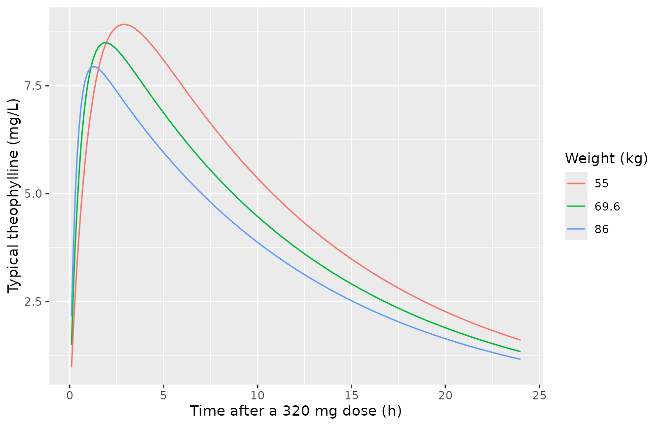
Weight effect
Body weight enters as (WT / 69.6)^2.55 on ka and
(WT / 69.6)^0.57 on V. The large ka exponent mainly moves
the absorption phase.
# zeroRe() on a several-subject event table makes rxode2 warn that it is
# simulating without omega; that is the intent here, so only that warning is
# muffled.
muffle_no_omega <- function(w) {
  if (grepl("without 'omega'", conditionMessage(w), fixed = TRUE)) {
    invokeRestart("muffleWarning")
  }
}
solve_typical <- function(m, ev) {
  withCallingHandlers(
    rxode2::rxSolve(rxode2::zeroRe(m), events = ev, keep = "WT"),
    warning = muffle_no_omega
  )
}

wts <- c(55, wt_ref, 86)
ev_wt <- dplyr::bind_rows(lapply(seq_along(wts), function(i) {
  dplyr::bind_rows(
    data.frame(id = i, time = 0, evid = 1L, amt = 320, cmt = "depot", WT = wts[i]),
    data.frame(id = i, time = seq(0.1, 24, by = 0.1), evid = 0L, amt = 0, cmt = "central", WT = wts[i])
  )
}))
sim_wt <- solve_typical(mod_theo, ev_wt)
#> ℹ parameter labels from comments will be replaced by 'label()'
#> ℹ omega/sigma items treated as zero: 'etalka', 'etalkel', 'etalvc'
ggplot(as.data.frame(sim_wt), aes(time, Cc, colour = factor(round(WT, 1)))) +
  geom_line() +
  labs(
    x = "Time after a 320 mg dose (h)", y = "Typical theophylline (mg/L)",
    colour = "Weight (kg)"
  )
Agreement with the SAEM-based fits
Table 1 reports the same covariate model from COSSAC and SCM
(identical columns: ka 1.60, ke 0.087, V 31.82, beta_ka,w
2.58, beta_V,w 0.57). The typical profiles of the VAE and
COSSAC/SCM estimates are nearly identical, as the paper reports.
mod_cossac <- mod_theo |>
  rxode2::ini(lka = log(1.60), lkel = log(0.087), lvc = log(31.82), e_wt_ka = 2.58)
#> ℹ parameter labels from comments will be replaced by 'label()'
#> ℹ change initial estimate of `lka` to `0.470003629245736`
#> ℹ change initial estimate of `lkel` to `-2.44184716032755`
#> ℹ change initial estimate of `lvc` to `3.46009502290964`
#> ℹ change initial estimate of `e_wt_ka` to `2.58`
sim_cossac <- solve_typical(mod_cossac, ev_wt)
#> ℹ omega/sigma items treated as zero: 'etalka', 'etalkel', 'etalvc'
max_rel <- max(abs(sim_cossac$Cc / sim_wt$Cc - 1))
max_rel
#> [1] 0.01966659
# Deterministic: measured 0.020, from the small differences in ka, ke and V and
# the 0.03 difference in the ka weight exponent across the three weights.
stopifnot(max_rel < 0.03)
Neonatal weight change
Equation 15 solved independently
The packaged model is compared with a fixed-step fourth-order Runge-Kutta integration of Equation 15 written directly from the paper.
mod_neo <- readModelDb("Rohleff_2025_neonatalWeight")

eq15_rhs <- function(t, w, p) {
  kprod <- p$kin / (1 + exp(-2 * (t - p$tlag)))
  kelim <- p$kout * (1 - t / (p$t50 + t))
  kprod - kelim * w
}
rk4_eq15 <- function(p, t_end, h) {
  n <- round(t_end / h)
  w <- numeric(n + 1)
  w[1] <- p$w0
  for (i in seq_len(n)) {
    t <- (i - 1) * h
    k1 <- eq15_rhs(t, w[i], p)
    k2 <- eq15_rhs(t + h / 2, w[i] + h / 2 * k1, p)
    k3 <- eq15_rhs(t + h / 2, w[i] + h / 2 * k2, p)
    k4 <- eq15_rhs(t + h, w[i] + h * k3, p)
    w[i + 1] <- w[i] + h / 6 * (k1 + 2 * k2 + 2 * k3 + k4)
  }
  data.frame(time = seq(0, by = h, length.out = n + 1), w = w)
}

p_vae <- list(w0 = 3383.2, kin = 106.8, tlag = 1.56, kout = 0.072, t50 = 1.18)
ref <- rk4_eq15(p_vae, t_end = 7, h = 0.001)

ev_neo <- data.frame(id = 1L, time = seq(0, 7, by = 0.01), evid = 0L, amt = 0, cmt = "bw")
typ_neo <- as.data.frame(rxode2::rxSolve(
  rxode2::zeroRe(mod_neo), events = ev_neo, rtol = 1e-10, atol = 1e-10
))
#> ℹ parameter labels from comments will be replaced by 'label()'
#> ℹ omega/sigma items treated as zero: 'etalrbase', 'etalkin', 'etalkin_t50', 'etalkout', 'etalkout_t50'
ref_at <- ref$w[match(round(typ_neo$time, 3), round(ref$time, 3))]
stopifnot(!anyNA(ref_at))
rk4_err <- max(abs(typ_neo$bw / ref_at - 1))
rk4_err
#> [1] 2.230955e-10
stopifnot(rk4_err < 1e-7)
Typical trajectory: VAE vs SAEM estimates
Table S3 reports the covariate-free fit by both the VAE and SAEM. The two parameter sets give almost the same typical course: a loss of about 6% of birth weight with the nadir a little after day 2, and birth weight regained before day 7.
mod_neo_saem <- mod_neo |>
  rxode2::ini(
    lrbase = log(3386.2), lkin = log(99.6), lkin_t50 = log(1.61),
    lkout = log(0.076), lkout_t50 = log(0.9)
  )
#> ℹ parameter labels from comments will be replaced by 'label()'
#> ℹ change initial estimate of `lrbase` to `8.12746362769413`
#> ℹ change initial estimate of `lkin` to `4.60116216459055`
#> ℹ change initial estimate of `lkin_t50` to `0.476234178996372`
#> ℹ change initial estimate of `lkout` to `-2.57702193869581`
#> ℹ change initial estimate of `lkout_t50` to `-0.105360515657826`
typ_saem <- as.data.frame(rxode2::rxSolve(
  rxode2::zeroRe(mod_neo_saem), events = ev_neo, rtol = 1e-10, atol = 1e-10
))
#> ℹ omega/sigma items treated as zero: 'etalrbase', 'etalkin', 'etalkin_t50', 'etalkout', 'etalkout_t50'

summarise_course <- function(d, w0) {
  i <- which.min(d$bw)
  data.frame(
    nadir_day = d$time[i],
    nadir_pct = 100 * (d$bw[i] / w0 - 1),
    day7_pct = 100 * (d$bw[nrow(d)] / w0 - 1),
    regain_day = d$time[which(d$time > d$time[i] & d$bw >= w0)[1]]
  )
}
course <- dplyr::bind_rows(
  cbind(Fit = "VAE (packaged)", summarise_course(typ_neo, 3383.2)),
  cbind(Fit = "SAEM", summarise_course(typ_saem, 3386.2))
)
course |>
  dplyr::rename(
    "Nadir (day)" = nadir_day, "Nadir (% of W0)" = nadir_pct,
    "Day 7 (% of W0)" = day7_pct, "Birth weight regained (day)" = regain_day
  ) |>
knitr::kable(digits = 2, caption = "Typical weight course from the two Table S3 parameter sets.")| Fit | Nadir (day) | Nadir (% of W0) | Day 7 (% of W0) | Birth weight regained (day) |
|---|---|---|---|---|
| VAE (packaged) | 2.14 | -6.26 | 1.27 | 6.39 |
| SAEM | 2.10 | -6.09 | 1.47 | 6.28 |
# Deterministic regression checks on the packaged (VAE) typical course:
# measured nadir -6.26% at day 2.14; a transcription error in any of the five
# parameters moves these well beyond the bounds.
vae <- course[course$Fit == "VAE (packaged)", ]
stopifnot(
  abs(vae$nadir_pct - (-6.26)) < 0.05,
  abs(vae$nadir_day - 2.14) < 0.02,
  abs(vae$nadir_pct - course$nadir_pct[course$Fit == "SAEM"]) < 0.5
)

dplyr::bind_rows(
  dplyr::mutate(typ_neo, Fit = "VAE (packaged)"),
  dplyr::mutate(typ_saem, Fit = "SAEM")
) |>
  ggplot(aes(time, bw, colour = Fit)) +
  geom_line() +
  labs(x = "Postnatal age (days)", y = "Typical body weight (g)")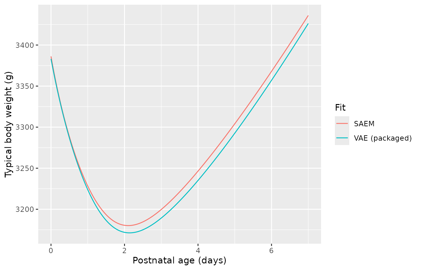
Simulated variability
There are no public observations to overlay, so this shows the spread the model implies for 200 virtual neonates, in grams and as percent change from each neonate’s own birth weight.
n_neo <- 200L
neo_events <- data.frame(id = seq_len(n_neo)) |>
  tidyr::crossing(time = seq(0, 7, by = 0.25)) |>
  dplyr::mutate(evid = 0L, amt = 0, cmt = "bw")
rxode2::rxSetSeed(20252)
sim_neo <- as.data.frame(rxode2::rxSolve(mod_neo, events = neo_events)) |>
  dplyr::group_by(id) |>
  dplyr::mutate(pct = 100 * (bw / bw[time == 0] - 1)) |>
  dplyr::ungroup()
#> ℹ parameter labels from comments will be replaced by 'label()'

sim_neo |>
  tidyr::pivot_longer(c(bw, pct), names_to = "scale", values_to = "value") |>
  dplyr::mutate(scale = ifelse(scale == "bw", "Body weight (g)", "Change from birth weight (%)")) |>
  dplyr::group_by(scale, time) |>
  dplyr::summarise(
    Q05 = quantile(value, 0.05), Q50 = median(value), Q95 = quantile(value, 0.95),
    .groups = "drop"
  ) |>
  ggplot(aes(time, Q50)) +
  geom_ribbon(aes(ymin = Q05, ymax = Q95), alpha = 0.25, fill = "darkorange") +
  geom_line(colour = "darkorange") +
  facet_wrap(~scale, scales = "free_y") +
  labs(x = "Postnatal age (days)", y = NULL, caption = "5th-50th-95th percentiles, 200 virtual neonates.")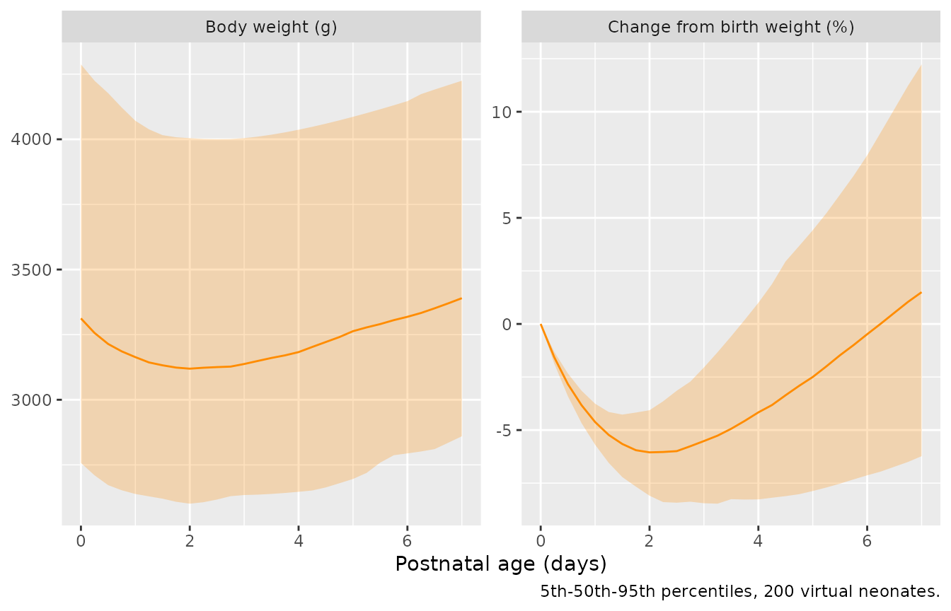
nadirs <- sim_neo |>
  dplyr::group_by(id) |>
  dplyr::summarise(nadir_pct = min(pct), .groups = "drop")
median(nadirs$nadir_pct)
#> [1] -6.10586
# Centre of the per-neonate nadir distribution; it sits near the typical
# -6.3% because the IIV is moderate. A wrong kout or kin moves it by several
# percentage points.
stopifnot(abs(median(nadirs$nadir_pct) - (-6.3)) < 1.5)
Assumptions and deviations
- Which estimates. Both models use the VAE column, the paper’s own method. Table 1 also gives COSSAC, SAMBA and SCM estimates for theophylline and Table S3 gives SAEM estimates for the neonates; they are shown above as comparisons.
-
Theophylline weight reference. The paper normalises
weight by “the mean weight over the N individuals” without printing it.
69.583 kg is the mean of the 12 weights in the authors’ deposited
dataset, which are those of
datasets::Theoph. -
Theophylline sex. Sex was offered on all three
parameters and every method dropped it; it is recorded in
covariatesDataExcluded(the paper codes male = 1). -
SAMBA column. The Results text says SAMBA “suggests
only the covariate effect
beta_V,w”, but Table 1 prints a SAMBA value forbeta_ka,w(2.53) and none forbeta_V,w. The packaged model does not use the SAMBA column, so the inconsistency does not affect it. -
Observed pre-dose samples.
datasets::Theophhas small non-zero concentrations at time zero; the authors’ fitted dataset has no time-zero records. For the NCA reference they are set to zero, consistent with the single-dose model. -
Neonatal covariate model not packaged. The VAE
retained covariate effects (Figure 4: sex, mode of delivery, gestational
age and parity on W0; sex, mode of delivery, gestational age, maternal
age and parity on kin; maternal age and parity on Tlag; maternal age on
kout; gestational age on T50), but the paper prints only their
convergence traces (Figure 5) and never the fixed effects or omegas of
the covariate model. The model cannot be reconstructed from the paper,
so the covariate-free fit of Table S3, which is fully reported, is
packaged instead. The selected covariates are listed in
covariatesDataExcluded; the paper does not state how sex, mode of delivery or parity were coded. -
Neonatal parameter names. The paper’s
Tlag(the midpoint of the smoothed onset of weight gain) iskin_t50and itsT50(the age at which the fractional loss rate has halved) iskout_t50, following the library’s<parameter>_t50naming for time-varying parameters. The steepness 2 per day of the onset sigmoid is a fixed constant of Equation 15, not an estimate. - Units. Time is in days and weight in grams for the neonatal model (Table S3 values, e.g. W0 = 3383.2); the paper states neither explicitly.
- No erratum or correction to the paper was found on EuropePMC as of 2026-11-11.