Diroximel fumarate metabolites MMF and HES (Kuchimanchi 2022)

Model and source

• Citation: Kuchimanchi M, Bockbrader H, Dolphin N, Epling D, Quinlan L, Chapel S, Penner N. Development of a Population Pharmacokinetic Model for the Diroximel Fumarate Metabolites Monomethyl Fumarate and 2-Hydroxyethyl Succinimide Following Oral Administration of Diroximel Fumarate in Healthy Participants and Patients with Multiple Sclerosis. Neurol Ther. 2022;11(1):353-371. doi:10.1007/s40120-021-00316-6
• Description: Joint population PK model for the two diroximel fumarate (DRF) metabolites, monomethyl fumarate (MMF, the active moiety) and 2-hydroxyethyl succinimide (HES, inactive), after oral DRF in 341 healthy volunteers and 48 patients with relapsing-remitting multiple sclerosis across 11 phase I and III studies. DRF itself is not measurable in plasma, so each dose enters two parallel absorption chains as its molar equivalent of MMF and of HES; each chain is a dose compartment followed by eight transit compartments (nine first-order transfers at the metabolite’s absorption rate constant) into a one-compartment disposition with first-order elimination. One central volume is shared by both metabolites; HES bioavailability is fixed at 0.6 from a mass-balance study and MMF bioavailability is estimated relative to it. Body weight scales both clearances and the volume, baseline eGFR scales HES clearance, and patients with MS have lower clearance of both metabolites. Meal fat content and evening dosing slow absorption, meal fat content lowers MMF bioavailability, and HES absorption carries a lag after an evening dose or a low-fat meal. The log-scale residual error is stratified by metabolite, meal state and dose time.
• Article: Neurol Ther 2022;11(1):353-371 (open access)
• Supplement: Electronic Supplementary Material 1 (supplementary methods and results, the final-model NONMEM control stream, and Tables S1-S6), available from the article page.

Diroximel fumarate (DRF) is an oral prodrug for relapsing multiple sclerosis. It is split presystemically into monomethyl fumarate (MMF), the active moiety that DRF shares with dimethyl fumarate, and 2-hydroxyethyl succinimide (HES), an inactive metabolite. DRF itself cannot be measured in plasma, so the model treats each dose as its molar equivalent of MMF and of HES, each absorbed through its own transit chain into a one-compartment disposition. The two metabolites share one central volume.

Population

The analysis pooled 4694 MMF and 8088 HES plasma concentrations from 389 participants in 11 studies: 341 healthy volunteers in nine phase I studies (including 32 participants with normal to severely impaired renal function in study A108) and 48 patients with relapsing-remitting multiple sclerosis in the phase III EVOLVE-MS-1 and EVOLVE-MS-2 studies (Table 1; Results, Study Population). Median age was 35 years (range 18-75), 49.4% were female, 66.3% were White and 30.8% Black, and median body weight was 78 kg (range 47.4-126.3 kg). By MDRD eGFR, 75.5% had normal renal function and 20.0%, 2.3% and 2.0% had mild, moderate and severe impairment (ESM Tables S1-S2). Doses ranged from 49 to 980 mg DRF; 69% received the approved 462 mg dose. Healthy participants were dosed fasted (n = 252) or with a low-fat (n = 47), medium-fat (n = 47) or high-fat (n = 58) meal; the patients took DRF with or without food, so their meal state is unknown.

The same information is available programmatically via readModelDb("Kuchimanchi_2022_diroximelFumarate")()$population.

Source trace

Values come from Table 2 of the article and the final-model NONMEM control stream in the ESM. Theta numbers are those of the control stream.

Equation / parameter	Value	Source location
lcl (CLMMF)	log(13.5 L/h)	Table 2, theta 1
lvc (Vc, shared)	log(30.4 L)	Table 2, theta 2; stream V3 = V2
lka (KaMMF)	log(5.04 1/h)	Table 2, theta 3
lka_hes (KaHES)	log(3.24 1/h)	Table 2, theta 6
lcl_hes (CLHES)	log(1.49 L/h)	Table 2, theta 7
lfdepot_hes (F4)	fixed(log(0.6))	Table 2, theta 8 (FIXED; mass-balance study)
lfdepot (F1)	log(0.162)	Table 2, theta 9
e_wt_vc	0.878	Table 2, theta 10
e_crcl_cl_hes	0.547	Table 2, theta 26
e_wt_cl	0.831	Table 2, theta 27 (row mislabelled ‘eGFR on CLHES’)
e_wt_cl_hes	0.335	Table 2, theta 28
e_patient_cl, e_patient_cl_hes	-0.284, -0.122	Table 2, thetas 35-36
e_dosetime_evening_ka, e_fed_lowfat_ka, e_fed_medfat_ka, e_fed_highfat_ka	-0.592, -0.368, -0.512, -0.666 (all FIXED)	Table 2, thetas 11-14
e_fed_missing_ka	0.843	Table 2, theta 15
e_fed_lowfat_fdepot, e_fed_medfat_fdepot, e_fed_highfat_fdepot	-0.296, -0.301, -0.131 (all FIXED)	Table 2, thetas 16-18 (theta 17 mislabelled ‘LOW on F1’)
e_dosetime_evening_ka_hes, e_fed_lowfat_ka_hes, e_fed_medfat_ka_hes, e_fed_highfat_ka_hes	-0.267, -0.335, -0.492, -0.621 (all FIXED)	Table 2, thetas 19-22
e_fed_missing_ka_hes	0.399	Table 2, theta 23
e_dosetime_evening_tlag_hes, e_fed_lowfat_tlag_hes	1.96 h, 0.421 h (FIXED)	Table 2, thetas 24-25
etalcl, etalvc, etalcl_hes	0.237^2, 0.198^2, 0.180^2	Table 2 IIV (%CV = sqrt(omega^2) x 100, ESM)
etalka, etalka_hes	0.370^2, 0.424^2	Table 2 IIV (KaMMF row mislabelled ‘ETA4-CLHES’)
expSd, expSdFed, expSdEvening, expSdFedMissing	0.895, 1.03, 1.12, 1.02	Table 2, thetas 4, 29-31
expSd_hes, expSdFed_hes, expSdEvening_hes, expSdFedMissing_hes	0.252, 0.468, 0.184, 0.372	Table 2, thetas 5, 32-34
Clearances, volume, Ka, F1 covariate equations	n/a	Table 2 ‘Model equations’; stream $PK
Nine first-order transfers per analyte (dose compartment + 8 transits)	n/a	Fig. 1a; stream $MODEL and K15 … K19T2, K46 … K20T3
Molar-equivalent dose input	n/a	Results, Model Development
HES lag ALAG4 = PM1 * theta24 + BFAT1 * theta25	n/a	stream $PK
Log-scale residual, SD stratified by metabolite, meal and dose time	n/a	ESM Methods; stream $ERROR

Dosing and helpers

Each DRF dose is given in milligrams to both depot (MMF chain) and depot_hes (HES chain). The model multiplies each by the molar ratio of the metabolite to DRF (130.10 / 255.22 for MMF, 143.14 / 255.22 for HES) and by the bioavailability, so concentrations come out in ug/mL. Observation rows use dvid = 1 because the model has two error endpoints; both Cc (MMF) and Cc_hes come back as columns.

mod <- readModelDb("Kuchimanchi_2022_diroximelFumarate")
mod_typical <- rxode2::zeroRe(mod)
#> ℹ parameter labels from comments will be replaced by 'label()'
#> Warning: No sigma parameters in the model

mw_ratio_mmf <- 130.10 / 255.22
mw_ratio_hes <- 143.14 / 255.22

# Reference participant of the paper's simulations: 78 kg, eGFR 111.9 mL/min,
# healthy, fasted, morning dose.
set_covariates <- function(ev, WT = 78, CRCL = 111.9, DIS_HEALTHY = 1,
                           FED_LOWFAT = 0, FED_MEDFAT = 0, FED_HIGHFAT = 0,
                           FED_MISSING = 0) {
  ev$WT <- WT
  ev$CRCL <- CRCL
  ev$DIS_HEALTHY <- DIS_HEALTHY
  ev$FED_LOWFAT <- FED_LOWFAT
  ev$FED_MEDFAT <- FED_MEDFAT
  ev$FED_HIGHFAT <- FED_HIGHFAT
  ev$FED_MISSING <- FED_MISSING
  ev
}

# 462 mg DRF twice daily for 7 days (14 doses, the design of Figs. 2 and 3),
# observing the final 24 h. `evening_alternate = TRUE` flags every second dose
# (and the records that follow it until the next morning dose) as an evening
# dose; otherwise every dose is a morning dose.
bid_events <- function(ids, obs_times = seq(144, 168, by = 0.05),
                       evening_alternate = FALSE, amt = 462) {
  dose_times <- seq(0, by = 12, length.out = 14)
  one <- dplyr::bind_rows(
    data.frame(
      time = rep(dose_times, each = 2), evid = 1L, amt = amt,
      cmt = rep(c("depot", "depot_hes"), length(dose_times)), dvid = NA_integer_
    ),
    data.frame(time = obs_times, evid = 0L, amt = 0, cmt = "central", dvid = 1L)
  )
  one$DOSETIME_EVENING <- if (evening_alternate) {
    as.integer((one$time %% 24) >= 12)
  } else {
    0L
  }
  ev <- tidyr::expand_grid(id = ids, one) |>
    dplyr::arrange(id, time, dplyr::desc(evid))
  ev[, c("id", "time", "evid", "amt", "cmt", "dvid", "DOSETIME_EVENING")]
}

interval_summary <- function(sim, lo, hi) {
  sim |>
    dplyr::filter(time >= lo, time <= hi) |>
    dplyr::group_by(id) |>
    dplyr::summarise(
      cmax_mmf = max(Cc), tmax_mmf = time[which.max(Cc)] - lo,
      auc_mmf = sum(diff(time) * (head(Cc, -1) + tail(Cc, -1)) / 2),
      cmax_hes = max(Cc_hes), tmax_hes = time[which.max(Cc_hes)] - lo,
      auc_hes = sum(diff(time) * (head(Cc_hes, -1) + tail(Cc_hes, -1)) / 2),
      .groups = "drop"
    )
}

Replicate Figure 3A: typical MMF profiles by meal state

Figure 3A shows the steady-state MMF profile after the morning dose on day 7 of 462 mg DRF twice daily, for a 78 kg healthy participant dosed fasted or with a low-, medium- or high-fat meal, and for a patient with MS (unknown meal state). The reference values below were read from the figure by the maintainers (peak height to about 0.02 ug/mL, peak time to about 0.2 h).

conditions <- tibble::tribble(
  ~id, ~condition, ~DIS_HEALTHY, ~FED_LOWFAT, ~FED_MEDFAT, ~FED_HIGHFAT, ~FED_MISSING,
  1L, "Fasted (HV)", 1, 0, 0, 0, 0,
  2L, "Low fat (HV)", 1, 1, 0, 0, 0,
  3L, "Medium fat (HV)", 1, 0, 1, 0, 0,
  4L, "High fat (HV)", 1, 0, 0, 1, 0,
  5L, "Unknown (patient)", 0, 0, 0, 0, 1
)

ev_3a <- dplyr::left_join(
  bid_events(conditions$id),
  conditions,
  by = "id"
)
ev_3a$WT <- 78
ev_3a$CRCL <- 111.9

sim_3a <- rxode2::rxSolve(mod_typical, events = ev_3a, keep = "condition") |>
  as.data.frame()
#> ℹ omega/sigma items treated as zero: 'etalcl', 'etalvc', 'etalcl_hes', 'etalka', 'etalka_hes'
#> Warning: multi-subject simulation without without 'omega'

typ_3a <- interval_summary(sim_3a, 144, 156) |>
  dplyr::left_join(conditions[, c("id", "condition")], by = "id")

fig3a_ref <- tibble::tribble(
  ~condition, ~cmax_ref, ~tmax_ref,
  "Fasted (HV)", 0.77, 2.5,
  "Low fat (HV)", 0.45, 3.7,
  "Medium fat (HV)", 0.40, 4.7,
  "High fat (HV)", 0.40, 6.4,
  "Unknown (patient)", 1.00, 1.6
)
cmp_3a <- dplyr::inner_join(typ_3a, fig3a_ref, by = "condition")
stopifnot(nrow(cmp_3a) == 5L)

cmp_3a |>
  dplyr::transmute(
    condition,
    cmax_sim = signif(cmax_mmf, 3), cmax_ref,
    tmax_sim = round(tmax_mmf, 2), tmax_ref
  ) |>
  dplyr::rename(
    "Condition" = condition,
    "Cmax simulated (ug/mL)" = cmax_sim, "Cmax Fig. 3A (ug/mL)" = cmax_ref,
    "Tmax simulated (h)" = tmax_sim, "Tmax Fig. 3A (h)" = tmax_ref
  ) |>
  knitr::kable(caption = "Typical steady-state MMF peak after the day-7 morning dose.")

Typical steady-state MMF peak after the day-7 morning dose.

Condition	Cmax simulated (ug/mL)	Cmax Fig. 3A (ug/mL)	Tmax simulated (h)	Tmax Fig. 3A (h)
Fasted (HV)	0.772	0.77	2.50	2.5
Low fat (HV)	0.454	0.45	3.70	3.7
Medium fat (HV)	0.399	0.40	4.60	4.7
High fat (HV)	0.403	0.40	6.30	6.4
Unknown (patient)	1.000	1.00	1.55	1.6

# Deterministic typical-value solve: the only uncertainty is reading the figure.
stopifnot(
  all(abs(cmp_3a$cmax_mmf / cmp_3a$cmax_ref - 1) < 0.08),
  all(abs(cmp_3a$tmax_mmf - cmp_3a$tmax_ref) < 0.4)
)

The peak times are what pin the absorption chain. The control stream moves each dose through nine first-order transfers at Ka (a dose compartment and eight transit compartments). With one transfer fewer, the typical fasted and patient peaks would arrive at 2.26 h and 1.40 h instead of the 2.5 h and 1.6 h the figure shows.

sim_3a |>
  dplyr::filter(time >= 144, time <= 156) |>
  ggplot(aes(time - 144, Cc, colour = condition, linetype = condition)) +
  geom_line(linewidth = 0.8) +
  labs(
    x = "Time after the day-7 morning dose (h)", y = "MMF concentration (ug/mL)",
    colour = NULL, linetype = NULL,
    title = "Figure 3A - typical steady-state MMF profiles, 462 mg DRF BID",
    caption = "Replicates Figure 3A of Kuchimanchi 2022 (78 kg, eGFR 111.9 mL/min)."
  ) +
  theme_bw()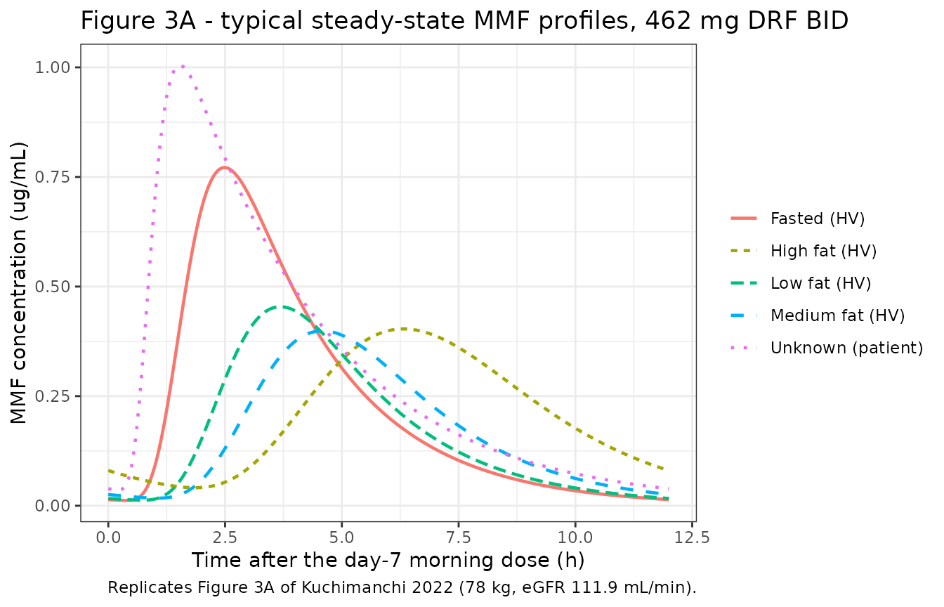

The same simulation for HES (not shown in the paper) illustrates why food barely changes HES: its half-life of about 14 h smooths out the slower absorption, and food does not change its bioavailability.

sim_3a |>
  dplyr::filter(time >= 144, time <= 156) |>
  ggplot(aes(time - 144, Cc_hes, colour = condition, linetype = condition)) +
  geom_line(linewidth = 0.8) +
  labs(
    x = "Time after the day-7 morning dose (h)", y = "HES concentration (ug/mL)",
    colour = NULL, linetype = NULL,
    title = "Typical steady-state HES profiles, 462 mg DRF BID"
  ) +
  theme_bw()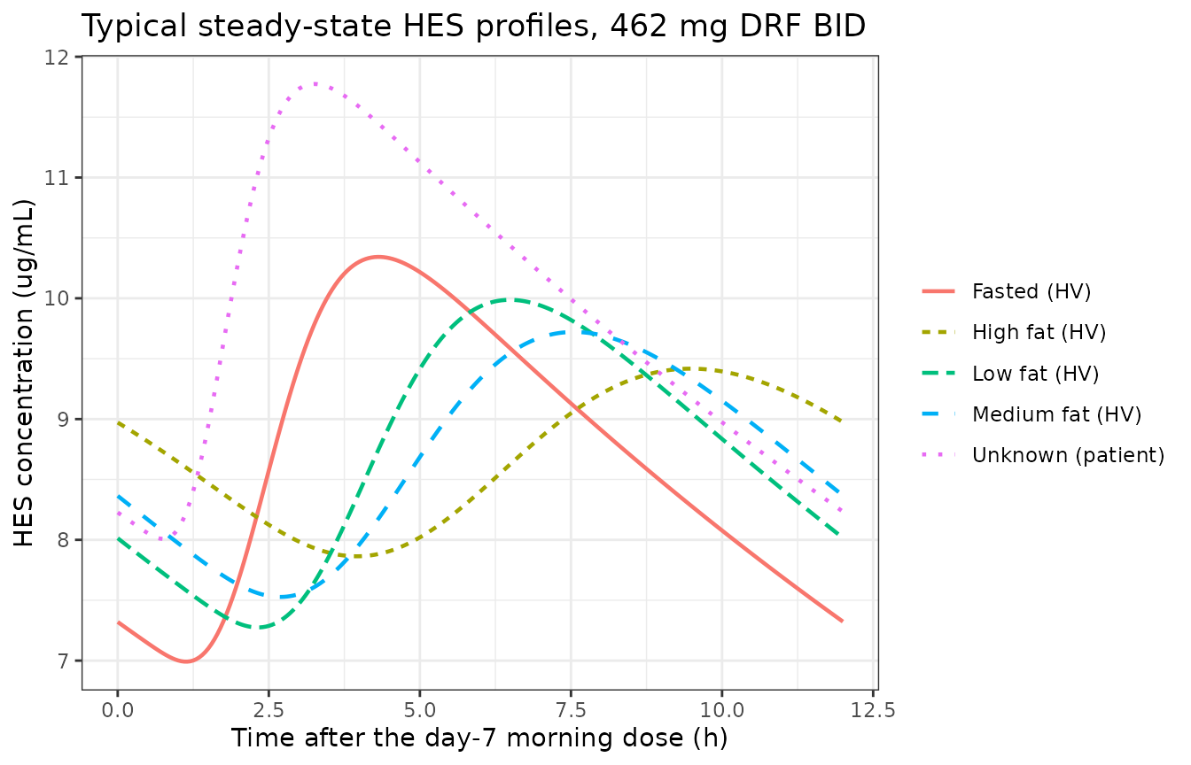

Replicate Figure 3B and steady-state NCA with PKNCA

Figure 3B shows the distribution of steady-state MMF Cmax after the morning dose for 1000 virtual participants per condition with between-subject variability, all at 78 kg and eGFR 111.9 mL/min. Here 200 participants per condition are simulated and NCA is run with PKNCA over the day-7 morning dosing interval (144-156 h). The reference medians were read from Figure 3B by the maintainers.

rxode2::rxSetSeed(20220118)
n_per_arm <- 200L

# Disjoint id ranges per condition: arm i holds ids (i - 1) * 200 + 1:200.
ev_3b <- bid_events(
  seq_len(nrow(conditions) * n_per_arm),
  obs_times = c(seq(132, 144, by = 1), seq(144.25, 156, by = 0.25))
) |>
  dplyr::mutate(arm = (id - 1L) %/% n_per_arm + 1L) |>
  dplyr::left_join(dplyr::rename(conditions, arm = id), by = "arm")
ev_3b$WT <- 78
ev_3b$CRCL <- 111.9
# Each subject belongs to exactly one condition, and each condition has 200.
stopifnot(
  !anyDuplicated(dplyr::distinct(ev_3b, id, condition)$id),
  all(table(dplyr::distinct(ev_3b, id, condition)$condition) == n_per_arm)
)

sim_3b <- rxode2::rxSolve(mod, events = ev_3b, keep = "condition") |>
  as.data.frame()
#> ℹ parameter labels from comments will be replaced by 'label()'
stopifnot(!anyNA(sim_3b$Cc), !anyNA(sim_3b$Cc_hes))

# Residual error is not part of Figure 3B: `Cc` and `Cc_hes` are the
# individual predictions (the simulated observations are in `sim`).
# Doses: one DRF dose per dosing time (the depot_hes record is the same dose).
dose_df <- ev_3b |>
  dplyr::filter(evid == 1, cmt == "depot") |>
  dplyr::select(id, time, amt, condition)

run_nca <- function(conc_col) {
  conc_df <- sim_3b |>
    dplyr::filter(!is.na(.data[[conc_col]]), time >= 132) |>
    dplyr::select(id, time, conc = dplyr::all_of(conc_col), condition)
  conc_obj <- PKNCA::PKNCAconc(conc_df, conc ~ time | condition + id)
  dose_obj <- PKNCA::PKNCAdose(dose_df, amt ~ time | condition + id)
  intervals <- data.frame(start = 144, end = 156, cmax = TRUE, tmax = TRUE, auclast = TRUE)
  PKNCA::pk.nca(PKNCA::PKNCAdata(conc_obj, dose_obj, intervals = intervals))
}
nca_mmf <- run_nca("Cc")
nca_hes <- run_nca("Cc_hes")

fig3b_ref <- tibble::tribble(
  ~condition, ~cmax,
  "Fasted (HV)", 0.77,
  "Low fat (HV)", 0.46,
  "Medium fat (HV)", 0.39,
  "High fat (HV)", 0.41,
  "Unknown (patient)", 1.01
)
cmp_3b <- nlmixr2lib::ncaComparisonTable(
  simulated = nca_mmf,
  reference = fig3b_ref,
  by = "condition",
  params = "cmax",
  units = c(cmax = "ug/mL"),
  tolerance_pct = 20
)
knitr::kable(
  cmp_3b,
  caption = paste(
    "Median steady-state MMF Cmax after the day-7 morning dose (simulated, 200",
    "per condition) vs Figure 3B medians. * differs from the reference by >20%."
  )
)

Median steady-state MMF Cmax after the day-7 morning dose (simulated, 200 per condition) vs Figure 3B medians. * differs from the reference by >20%.

NCA parameter	condition	Reference	Simulated	% diff
Cmax (ug/mL)	Fasted (HV)	0.77	0.755	-2.0%
Cmax (ug/mL)	Low fat (HV)	0.46	0.457	-0.7%
Cmax (ug/mL)	Medium fat (HV)	0.39	0.407	+4.3%
Cmax (ug/mL)	High fat (HV)	0.41	0.394	-4.0%
Cmax (ug/mL)	Unknown (patient)	1.01	0.998	-1.1%

cmax_med <- as.data.frame(nca_mmf) |>
  dplyr::filter(PPTESTCD == "cmax") |>
  dplyr::group_by(condition) |>
  dplyr::summarise(median_cmax = median(PPORRES), .groups = "drop") |>
  dplyr::inner_join(fig3b_ref, by = "condition")
stopifnot(nrow(cmax_med) == 5L)
# The median of 200 draws has a relative standard error of about 2-3% here;
# a mis-transcribed F1, Ka, CL or V moves it by tens of percent.
stopifnot(all(abs(cmax_med$median_cmax / cmax_med$cmax - 1) < 0.15))

as.data.frame(nca_mmf) |>
  dplyr::filter(PPTESTCD == "cmax") |>
  dplyr::mutate(condition = factor(condition, levels = conditions$condition)) |>
  ggplot(aes(condition, PPORRES)) +
  geom_boxplot(outlier.shape = NA) +
  geom_point(data = fig3b_ref, aes(condition, cmax), colour = "red", shape = 4, size = 3) +
  labs(
    x = NULL, y = "MMF Cmax,0-12h,ss (ug/mL)",
    title = "Figure 3B - steady-state MMF Cmax by meal state",
    caption = "Boxes: simulated (200 per condition). Crosses: Figure 3B medians. Replicates Figure 3B of Kuchimanchi 2022."
  ) +
  theme_bw()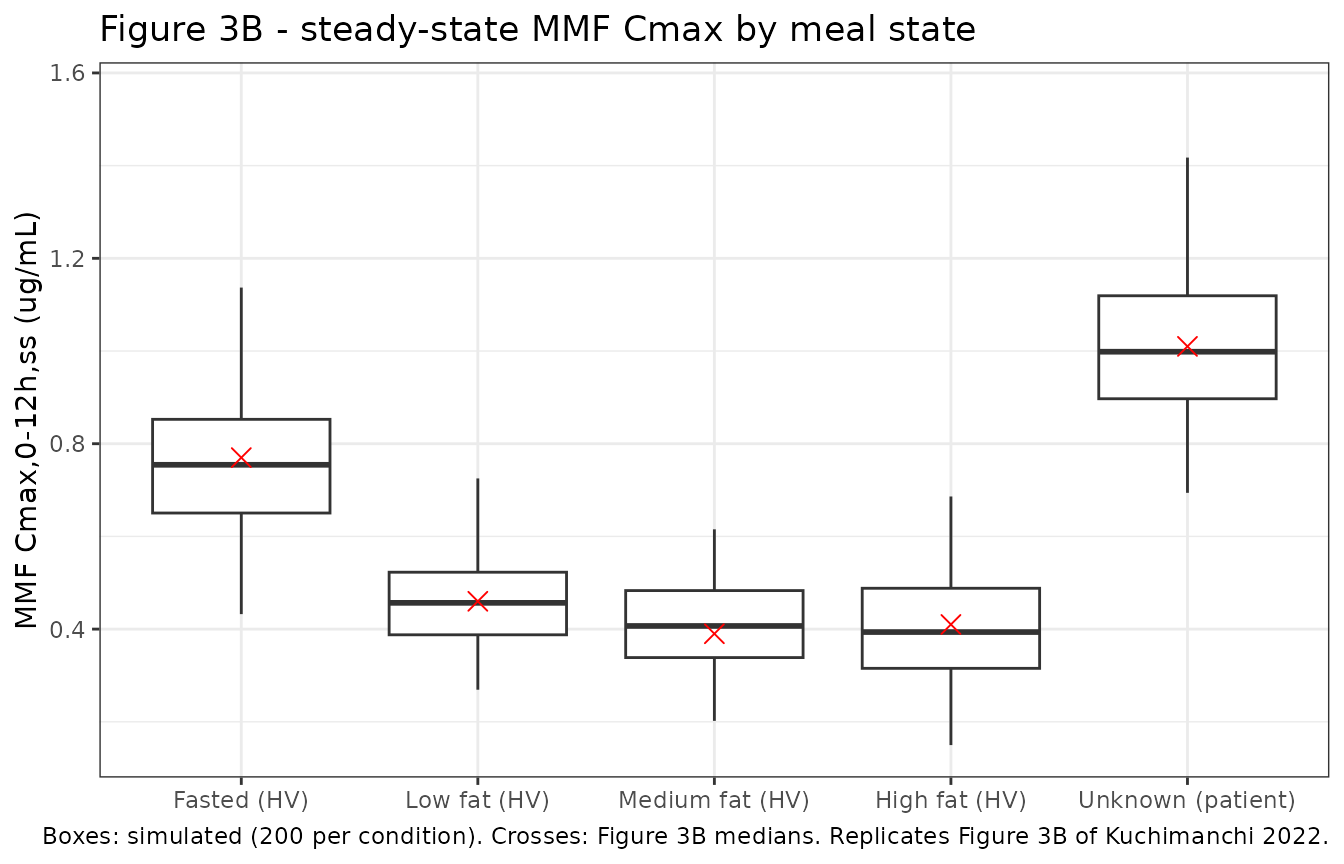

The paper reports no NCA table, so the HES and AUC results below have no published counterpart. They are shown for reference.

nca_summary <- dplyr::bind_rows(
  as.data.frame(nca_mmf) |> dplyr::mutate(analyte = "MMF"),
  as.data.frame(nca_hes) |> dplyr::mutate(analyte = "HES")
) |>
  dplyr::filter(PPTESTCD %in% c("cmax", "tmax", "auclast")) |>
  dplyr::group_by(analyte, condition, PPTESTCD) |>
  dplyr::summarise(median = signif(median(PPORRES), 3), .groups = "drop") |>
  tidyr::pivot_wider(names_from = PPTESTCD, values_from = median) |>
  dplyr::mutate(analyte = factor(analyte, levels = c("MMF", "HES"))) |>
  dplyr::arrange(analyte, condition)

nca_summary |>
  dplyr::rename(
    "Analyte" = analyte, "Condition" = condition,
    "Cmax (ug/mL)" = cmax, "Tmax (h)" = tmax, "AUC0-12h,ss (ug*h/mL)" = auclast
  ) |>
  knitr::kable(caption = "Median steady-state NCA over the day-7 morning dosing interval (200 per condition).")

Median steady-state NCA over the day-7 morning dosing interval (200 per condition).

Analyte	Condition	AUC0-12h,ss (ug*h/mL)	Cmax (ug/mL)	Tmax (h)
MMF	Fasted (HV)	2.78	0.755	2.50
MMF	High fat (HV)	2.37	0.394	6.00
MMF	Low fat (HV)	2.02	0.457	3.50
MMF	Medium fat (HV)	1.94	0.407	4.50
MMF	Unknown (patient)	3.91	0.998	1.75
HES	Fasted (HV)	102.00	10.000	4.50
HES	High fat (HV)	107.00	9.670	8.50
HES	Low fat (HV)	105.00	10.200	6.25
HES	Medium fat (HV)	103.00	9.710	7.25
HES	Unknown (patient)	118.00	11.700	3.25

Replicate Figure 2: covariate effects on steady-state exposure

Figure 2 plots the ratio of median steady-state Cmax and AUC0-12h under a test condition to the reference healthy participant (78 kg, eGFR 111.9 mL/min, fasted). Because every covariate enters multiplicatively on log-normally distributed parameters, the ratio of medians of AUC equals the typical-value ratio, so a typical-value solve is compared. The renal categories pool four test eGFR values each (Figure 2 legend); the median ratio of the four is used. Reference values: the Results text where it states a number, otherwise read from Figure 2 by the maintainers.

fig2_design <- tibble::tribble(
  ~test, ~WT, ~CRCL, ~FED_LOWFAT, ~FED_MEDFAT, ~FED_HIGHFAT,
  "Reference", 78, 111.9, 0, 0, 0,
  "Low fat meal", 78, 111.9, 1, 0, 0,
  "Medium fat meal", 78, 111.9, 0, 1, 0,
  "High fat meal", 78, 111.9, 0, 0, 1,
  "Body weight 55 kg", 55, 111.9, 0, 0, 0,
  "Body weight 100 kg", 100, 111.9, 0, 0, 0
) |>
  dplyr::bind_rows(tibble::tibble(
    test = rep(c("Normal renal function", "Mild renal impairment", "Moderate renal impairment", "Severe renal impairment"), each = 4),
    WT = 78,
    CRCL = c(120, 110, 100, 90, 89, 80, 70, 60, 59, 50, 40, 30, 29, 25, 20, 15),
    FED_LOWFAT = 0, FED_MEDFAT = 0, FED_HIGHFAT = 0
  )) |>
  dplyr::mutate(id = dplyr::row_number())

ev_2 <- bid_events(fig2_design$id, obs_times = seq(144, 156, by = 0.05)) |>
  dplyr::left_join(fig2_design, by = "id")
ev_2$DIS_HEALTHY <- 1
ev_2$FED_MISSING <- 0

sim_2 <- rxode2::rxSolve(mod_typical, events = ev_2, keep = "test") |>
  as.data.frame()
#> ℹ omega/sigma items treated as zero: 'etalcl', 'etalvc', 'etalcl_hes', 'etalka', 'etalka_hes'
#> Warning: multi-subject simulation without without 'omega'
ratios <- interval_summary(sim_2, 144, 156) |>
  dplyr::left_join(fig2_design[, c("id", "test")], by = "id")
ref_row <- ratios[ratios$test == "Reference", ]
ratios_2 <- ratios |>
  dplyr::mutate(
    r_cmax_mmf = cmax_mmf / ref_row$cmax_mmf, r_auc_mmf = auc_mmf / ref_row$auc_mmf,
    r_cmax_hes = cmax_hes / ref_row$cmax_hes, r_auc_hes = auc_hes / ref_row$auc_hes
  ) |>
  dplyr::group_by(test) |>
  dplyr::summarise(dplyr::across(dplyr::starts_with("r_"), median), .groups = "drop")

fig2_ref <- tibble::tribble(
  ~test, ~metric, ~reference, ~source,
  "Low fat meal", "r_cmax_mmf", 0.58, "Fig. 2A",
  "Medium fat meal", "r_cmax_mmf", 0.52, "Fig. 2A",
  "High fat meal", "r_cmax_mmf", 0.53, "Fig. 2A",
  "Low fat meal", "r_auc_mmf", 0.70, "Fig. 2A",
  "Medium fat meal", "r_auc_mmf", 0.70, "Fig. 2A",
  "High fat meal", "r_auc_mmf", 0.85, "Fig. 2A",
  "Body weight 55 kg", "r_auc_mmf", 1.32, "Results text (+32%)",
  "Body weight 100 kg", "r_auc_mmf", 0.81, "Results text (-19%)",
  "Body weight 55 kg", "r_cmax_mmf", 1.35, "Fig. 2A",
  "Body weight 100 kg", "r_cmax_mmf", 0.81, "Fig. 2A",
  "Low fat meal", "r_cmax_hes", 0.97, "Fig. 2B",
  "Medium fat meal", "r_cmax_hes", 0.94, "Fig. 2B",
  "High fat meal", "r_cmax_hes", 0.92, "Fig. 2B",
  "High fat meal", "r_auc_hes", 1.00, "Fig. 2B",
  "Body weight 55 kg", "r_auc_hes", 1.14, "Results text (+14%)",
  "Body weight 100 kg", "r_auc_hes", 0.92, "Results text (-8%)",
  "Normal renal function", "r_auc_hes", 1.04, "Fig. 2B",
  "Mild renal impairment", "r_auc_hes", 1.2, "Results text (1.2-fold)",
  "Moderate renal impairment", "r_auc_hes", 1.6, "Results text (1.6-fold)",
  "Severe renal impairment", "r_auc_hes", 2.33, "Fig. 2B (text: about 2-fold)",
  "Mild renal impairment", "r_cmax_hes", 1.2, "Results text (1.2-fold)",
  "Moderate renal impairment", "r_cmax_hes", 1.5, "Results text (1.5-fold)",
  "Severe renal impairment", "r_cmax_hes", 2.1, "Fig. 2B (text: about 2-fold)"
)

cmp_2 <- ratios_2 |>
  tidyr::pivot_longer(dplyr::starts_with("r_"), names_to = "metric", values_to = "simulated") |>
  dplyr::inner_join(fig2_ref, by = c("test", "metric"))
stopifnot(nrow(cmp_2) == nrow(fig2_ref))

metric_labels <- c(
  r_cmax_mmf = "MMF Cmax ratio", r_auc_mmf = "MMF AUC ratio",
  r_cmax_hes = "HES Cmax ratio", r_auc_hes = "HES AUC ratio"
)
cmp_2 |>
  dplyr::mutate(metric = metric_labels[metric], simulated = round(simulated, 2)) |>
  dplyr::select(test, metric, simulated, reference, source) |>
  dplyr::rename(
    "Test condition" = test, "Metric" = metric, "Simulated" = simulated,
    "Published" = reference, "Published source" = source
  ) |>
  knitr::kable(caption = "Steady-state exposure ratios vs the reference participant (Figure 2).")

Steady-state exposure ratios vs the reference participant (Figure 2).

Test condition	Metric	Simulated	Published	Published source
Body weight 100 kg	MMF Cmax ratio	0.81	0.81	Fig. 2A
Body weight 100 kg	MMF AUC ratio	0.81	0.81	Results text (-19%)
Body weight 100 kg	HES AUC ratio	0.92	0.92	Results text (-8%)
Body weight 55 kg	MMF Cmax ratio	1.35	1.35	Fig. 2A
Body weight 55 kg	MMF AUC ratio	1.34	1.32	Results text (+32%)
Body weight 55 kg	HES AUC ratio	1.12	1.14	Results text (+14%)
High fat meal	MMF Cmax ratio	0.52	0.53	Fig. 2A
High fat meal	MMF AUC ratio	0.87	0.85	Fig. 2A
High fat meal	HES Cmax ratio	0.91	0.92	Fig. 2B
High fat meal	HES AUC ratio	1.00	1.00	Fig. 2B
Low fat meal	MMF Cmax ratio	0.59	0.58	Fig. 2A
Low fat meal	MMF AUC ratio	0.70	0.70	Fig. 2A
Low fat meal	HES Cmax ratio	0.97	0.97	Fig. 2B
Medium fat meal	MMF Cmax ratio	0.52	0.52	Fig. 2A
Medium fat meal	MMF AUC ratio	0.70	0.70	Fig. 2A
Medium fat meal	HES Cmax ratio	0.94	0.94	Fig. 2B
Mild renal impairment	HES Cmax ratio	1.20	1.20	Results text (1.2-fold)
Mild renal impairment	HES AUC ratio	1.24	1.20	Results text (1.2-fold)
Moderate renal impairment	HES Cmax ratio	1.53	1.50	Results text (1.5-fold)
Moderate renal impairment	HES AUC ratio	1.64	1.60	Results text (1.6-fold)
Normal renal function	HES AUC ratio	1.04	1.04	Fig. 2B
Severe renal impairment	HES Cmax ratio	2.09	2.10	Fig. 2B (text: about 2-fold)
Severe renal impairment	HES AUC ratio	2.31	2.33	Fig. 2B (text: about 2-fold)

# Typical-value ratios against numbers stated in the text or read from the
# forest plot (read to about +/-0.03). The largest gap measured is 0.04 (the
# mild and moderate renal HES AUC against the rounded 1.2- and 1.6-fold of the
# text); a transcribed exponent or reference value off by 10% moves the
# weight and renal ratios by more than 0.1.
stopifnot(all(abs(cmp_2$simulated - cmp_2$reference) < 0.1))

The Results text also states the covariate effects on the parameters directly; these follow from the power exponents and are exact.

wt_param <- tibble::tribble(
  ~parameter, ~exponent, ~published_55kg, ~published_100kg,
  "CLMMF", 0.831, -25, 23,
  "CLHES", 0.335, -11, 9,
  "Vc", 0.878, -26, 24
) |>
  dplyr::mutate(
    simulated_55kg = round(100 * ((55 / 78)^exponent - 1)),
    simulated_100kg = round(100 * ((100 / 78)^exponent - 1))
  )
knitr::kable(wt_param, caption = "Percent change from the 78 kg participant (Results, Effect of Body Weight).")

Percent change from the 78 kg participant (Results, Effect of Body Weight).

parameter	exponent	published_55kg	published_100kg	simulated_55kg	simulated_100kg
CLMMF	0.831	-25	23	-25	23
CLHES	0.335	-11	9	-11	9
Vc	0.878	-26	24	-26	24

stopifnot(
  all(abs(wt_param$simulated_55kg - wt_param$published_55kg) <= 1),
  all(abs(wt_param$simulated_100kg - wt_param$published_100kg) <= 1)
)

Replicate Figure S2: morning versus evening dosing

ESM Figure S2 shows steady-state profiles for 462 mg twice daily with the second daily dose taken in the evening. The Results report that median Cmax,0-12h,ss after the evening dose is 37% lower for MMF and 12% lower for HES than after the morning dose. Here DOSETIME_EVENING alternates, set to 1 on each evening dose record and on the records that follow it until the next morning dose.

The evening HES lag is a covariate-driven alag(). To confirm that rxode2 applies each dose’s own lag and absorption rate, the alternating regimen is compared with the superposition of two separate solves, one of the morning doses only (flag 0 throughout) and one of the evening doses only (flag 1 throughout). The model is linear, so the two must agree.

ev_alt <- bid_events(1L, obs_times = seq(0, 168, by = 0.05), evening_alternate = TRUE) |>
  set_covariates()
ev_am <- bid_events(2L, obs_times = seq(0, 168, by = 0.05)) |>
  dplyr::filter(evid == 0 | (time %% 24) == 0) |>
  set_covariates()
ev_pm <- bid_events(3L, obs_times = seq(0, 168, by = 0.05)) |>
  dplyr::filter(evid == 0 | (time %% 24) == 12) |>
  dplyr::mutate(DOSETIME_EVENING = 1L) |>
  set_covariates()
sim_s2 <- rxode2::rxSolve(
  mod_typical,
  events = dplyr::bind_rows(ev_alt, ev_am, ev_pm)
) |>
  as.data.frame()
#> ℹ omega/sigma items treated as zero: 'etalcl', 'etalvc', 'etalcl_hes', 'etalka', 'etalka_hes'
#> Warning: multi-subject simulation without without 'omega'

alt <- sim_s2[sim_s2$id == 1, ]
sup <- sim_s2[sim_s2$id == 2, ]
sup$Cc <- sup$Cc + sim_s2$Cc[sim_s2$id == 3]
sup$Cc_hes <- sup$Cc_hes + sim_s2$Cc_hes[sim_s2$id == 3]
stopifnot(
  nrow(alt) == nrow(sup), isTRUE(all.equal(alt$time, sup$time)),
  max(abs(alt$Cc - sup$Cc)) / max(sup$Cc) < 1e-3,
  max(abs(alt$Cc_hes - sup$Cc_hes)) / max(sup$Cc_hes) < 1e-3
)

am_int <- interval_summary(alt, 144, 156)
pm_int <- interval_summary(alt, 156, 168)
s2 <- tibble::tibble(
  analyte = c("MMF", "HES"),
  simulated_pct = round(100 * (c(pm_int$cmax_mmf / am_int$cmax_mmf, pm_int$cmax_hes / am_int$cmax_hes) - 1)),
  published_pct = c(-37, -12)
)
s2 |>
  dplyr::rename(
    "Analyte" = analyte, "Simulated change in Cmax (%)" = simulated_pct,
    "Published change in median Cmax (%)" = published_pct
  ) |>
  knitr::kable(caption = "Evening vs morning steady-state Cmax (Results, Effect of Morning Versus Evening Dose).")

Evening vs morning steady-state Cmax (Results, Effect of Morning Versus Evening Dose).

Analyte	Simulated change in Cmax (%)	Published change in median Cmax (%)
MMF	-34	-37
HES	-13	-12

# Typical value (-34% / -13%) vs the median of an IIV simulation (-37% / -12%).
stopifnot(all(abs(s2$simulated_pct - s2$published_pct) <= 5))

alt |>
  dplyr::filter(time >= 144) |>
  tidyr::pivot_longer(c(Cc, Cc_hes), names_to = "analyte", values_to = "conc") |>
  dplyr::mutate(analyte = dplyr::recode(analyte, Cc = "MMF", Cc_hes = "HES")) |>
  ggplot(aes(time - 144, conc)) +
  geom_line(colour = "blue") +
  geom_vline(xintercept = 12, linetype = "dashed") +
  facet_wrap(~analyte, ncol = 1, scales = "free_y") +
  labs(
    x = "Time (h)", y = "Concentration (ug/mL)",
    title = "Figure S2 - morning (0 h) and evening (12 h) doses at steady state",
    caption = "Typical profile. Replicates ESM Figure S2 of Kuchimanchi 2022."
  ) +
  theme_bw()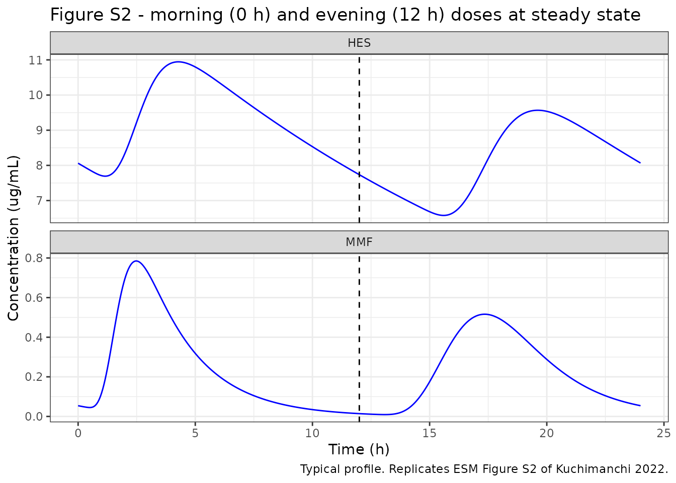

Mass balance at steady state

At steady state the exposure over one dosing interval must equal the absorbed molar-equivalent dose divided by clearance. This checks the dose conversion and bioavailability for each metabolite.

ref_int <- typ_3a[typ_3a$condition == "Fasted (HV)", ]
expected_auc_mmf <- 0.162 * 462 * mw_ratio_mmf / 13.5
expected_auc_hes <- 0.6 * 462 * mw_ratio_hes / 1.49
mass_balance <- tibble::tibble(
  analyte = c("MMF", "HES"),
  simulated = c(ref_int$auc_mmf, ref_int$auc_hes),
  expected = c(expected_auc_mmf, expected_auc_hes)
)
knitr::kable(mass_balance, digits = 3, caption = "AUC0-12h,ss (ug*h/mL) vs F x molar-equivalent dose / CL.")

AUC0-12h,ss (ug*h/mL) vs F x molar-equivalent dose / CL.

analyte	simulated	expected
MMF	2.826	2.826
HES	104.283	104.341

# Trapezoidal AUC on a 0.05 h grid; measured agreement better than 0.1%.
stopifnot(all(abs(mass_balance$simulated / mass_balance$expected - 1) < 0.005))

Assumptions and deviations

• Table 2 labels. Three rows of Table 2 carry the wrong label. Theta 27 (0.831) is labelled ‘eGFR on CLHES’ but is the body-weight exponent on MMF clearance; theta 17 (-0.301) is labelled ‘LOW on F1’ but is the medium-fat effect on F1; and the IIV row of 37.0 %CV is labelled ‘ETA4-CLHES’ but is ETA5, the IIV on KaMMF. The control-stream comments, the printed model equations and the Results text (‘37% for KaMMF’) agree on the corrected assignments.
• Absorption chain. The control stream moves each dose through nine transfers at Ka (dose compartment plus eight transits), so the mean absorption time is 9/Ka = 1.79 h for MMF and 2.78 h for HES. The Results quote 1.6 h and 2.5 h, which equal 8/Ka. The stream’s structure is implemented; the Figure 3A peak times confirm it.
• Dose units. The paper enters each DRF dose as its molar equivalent of MMF and of HES, with concentrations in mass units. The model takes DRF in mg and converts with molecular weights computed from the molecular formulae (DRF C11H13NO6, 255.22 g/mol; MMF C5H6O4, 130.10 g/mol; HES C6H9NO3, 143.14 g/mol); the paper does not print them. Figure 3A pins the choice: dosing DRF mg directly would double every MMF concentration.
• F1 is relative. MMF bioavailability (0.162) is estimated against a volume whose scale is set by HES, whose bioavailability is fixed at 0.6. It is not the absolute bioavailability of MMF.
• eGFR units. The eGFR covariate is the MDRD estimate denormalized to absolute mL/min with each participant’s body surface area (ESM Table S2), not the usual mL/min/1.73 m^2.
• Patient status. The source covariate PTST (1 = patient with MS) is carried as its complement DIS_HEALTHY. The paper notes that patient status and the unknown-meal stratum (FED_MISSING) cannot be separated, since only patients have an unknown meal state.
• Residual error in an unobserved stratum. The stream’s $ERROR block defines no residual SD for an evening dose taken with a known meal (there were no such records). The model uses the evening-dose SD for it.
• Time-varying covariates. The meal and dose-time indicators are read at every record, as in NONMEM. Hold them constant across a dosing interval and set them on the dose record and on the observations that follow it, as in the Figure S2 simulation above.
• Interoccasion variability. The final control stream fixes the IOV on KaMMF and KaHES to zero (ESM Results: IOV was not important), so it is not included.
• Figure readings. The Figure 2, 3A and 3B reference values were read from the published figures by the maintainers and carry about +/-0.02-0.03 of reading error.
• Errata. No correction notice for this article was found in Europe PMC as of 2026-09-30.