Cefiderocol in CRRT (Fouad 2024)
Source:vignettes/articles/Fouad_2024_cefiderocol.Rmd
Fouad_2024_cefiderocol.RmdModel and source
- Citation: Fouad A, Kobic E, Nicolasora NP, Thompson Bastin ML, Adams PM, Shen Y, Fratoni AJ, Ye X, Kuti JL, Nicolau DP, Asempa TE. Validation of cefiderocol package insert dosing recommendation for patients receiving continuous renal replacement therapy: a prospective multicenter pharmacokinetic study. Open Forum Infect Dis. 2024;11(10):ofae451. doi:10.1093/ofid/ofae451
- Description: Two-compartment population PK model for cefiderocol in critically ill adults on continuous venovenous haemodiafiltration (CVVHDF), fitted nonparametrically with the Pmetrics NPAG algorithm and parameterised by clearance, central volume and the intercompartmental micro-rate constants k12 and k21
- Article: https://doi.org/10.1093/ofid/ofae451 (PMC11492798; open access, CC BY)
- Supplement: Tables S1-S3 (eligibility, the label’s CRRT dosing table and the per-patient actual-versus-label exposure comparison) and Figures S1-S2 (covariate regressions and individual fits)
Cefiderocol is a siderophore cephalosporin whose United States label was the first to give antibiotic dosing by continuous renal replacement therapy (CRRT) effluent flow rate: 1.5 g q12h, 2 g q12h, 1.5 g q8h and 2 g q8h, each as a 3 h infusion, for effluent flows of at most 2, 2.1-3, 3.1-4 and at least 4.1 L/h. Fouad and colleagues ran a prospective three-centre study in critically ill adults on CRRT to validate those bands, fitting prefilter plasma concentrations nonparametrically with the NPAG algorithm in Pmetrics. The two-compartment base model they selected is the model packaged here.
Population
Fourteen ICU patients on continuous venovenous haemodiafiltration (CVVHDF, Prismaflex) were enrolled between August 2022 and December 2023 at Hartford Hospital (n = 7), Banner-University Medical Center (n = 5) and the University of Kentucky (n = 2). Five received cefiderocol for an actual or suspected infection and nine for PK sampling only. Five were dosed according to the label’s effluent-flow bands; nine had doses adjusted by the clinical team for obesity, residual renal function or an effluent flow that moved between bands (Supplementary Table S3). Prefilter samples were drawn after at least two prior doses at 0, 1.5, 3, 4, 6, 8 and (for q12h regimens) 12 h after the start of the dose.
knitr::kable(
  data.frame(
    Characteristic = c(
      "Patients", "Age (years)", "Male", "Weight (kg)", "BMI (kg/m^2)",
      "APACHE II", "Albumin (g/dL)", "Effluent flow (L/h)",
      "Effluent dose (mL/kg/h)", "Effluent band <= 2 / 2.1-3 / 3.1-4 / >= 4.1 L/h",
      "Regimens received", "Filters", "Fraction unbound"
    ),
    Value = c(
      "14", "55.4 +/- 14.9 (33-77)", "9 (64.3%)", "113.5 +/- 57.3 (62.4-265)",
      "37.6 +/- 16.2 (21-73)", "19 +/- 6.24 (10-32)", "3 +/- 0.6 (1.6-3.8)",
      "3.34 +/- 0.9 (2.08-5.1)", "32.7 +/- 10 (18-60)", "1 / 4 / 7 / 2",
      "2 g q6h (5), 2 g q8h (1), 1.5 g q8h (3), 2 g q12h (4), 1.5 g q12h (1)",
      "M100 (9), HF1400 (2), ST100 (3)", "0.84 +/- 0.1 (0.69-0.98)"
    )
  ),
  caption = "Fouad 2024 Table 1 and Results; mean +/- SD (range)."
)| Characteristic | Value |
|---|---|
| Patients | 14 |
| Age (years) | 55.4 +/- 14.9 (33-77) |
| Male | 9 (64.3%) |
| Weight (kg) | 113.5 +/- 57.3 (62.4-265) |
| BMI (kg/m^2) | 37.6 +/- 16.2 (21-73) |
| APACHE II | 19 +/- 6.24 (10-32) |
| Albumin (g/dL) | 3 +/- 0.6 (1.6-3.8) |
| Effluent flow (L/h) | 3.34 +/- 0.9 (2.08-5.1) |
| Effluent dose (mL/kg/h) | 32.7 +/- 10 (18-60) |
| Effluent band <= 2 / 2.1-3 / 3.1-4 / >= 4.1 L/h | 1 / 4 / 7 / 2 |
| Regimens received | 2 g q6h (5), 2 g q8h (1), 1.5 g q8h (3), 2 g q12h (4), 1.5 g q12h (1) |
| Filters | M100 (9), HF1400 (2), ST100 (3) |
| Fraction unbound | 0.84 +/- 0.1 (0.69-0.98) |
Source trace
knitr::kable(
  data.frame(
    Item = c(
      "lcl", "lvc", "lk12", "lk21",
      "etalcl / etalvc / etalk12 / etalk21",
      "addSd", "propSd",
      "Two-compartment ODE structure", "q, vp", "Cc", "Cfree", "FU",
      "WT, RRT_CRRT_EFFLUENT_FLOW, QEFF (excluded)"
    ),
    Value = c(
      "log(3.3) L/h", "log(7.4) L", "log(3.5) 1/h", "log(1.5) 1/h",
      "0.16043 / 0.48013 / 0.19311 / 0.69315",
      "0.0096 mg/L", "0.096",
      "central + peripheral1, micro-constants",
      "k12 * vc; q / k21", "central / vc", "FU * Cc", "0.84 (cohort mean)",
      "regressed on CL and Vc, not retained"
    ),
    Source = c(
      rep("Table 2, Median column", 4),
      "Table 2 SD / Mean, via omega^2 = log(1 + CV^2)",
      "Methods: SD = gamma x (0.006 + 0.06 x C); Results: gamma = 1.6",
      "Methods: SD = gamma x (0.006 + 0.06 x C); Results: gamma = 1.6",
      "Results: 2-compartment AIC 625.3 vs 1-compartment 656.9",
      "Algebraic identity of the Table 2 micro-constants",
      "Units: dose mg, vc L",
      "Methods 'Pharmacodynamic Analyses'",
      "Results 'Cefiderocol Exposures'",
      "Results 'Pharmacokinetics'; Supplementary Figure S1"
    )
  )
)| Item | Value | Source |
|---|---|---|
| lcl | log(3.3) L/h | Table 2, Median column |
| lvc | log(7.4) L | Table 2, Median column |
| lk12 | log(3.5) 1/h | Table 2, Median column |
| lk21 | log(1.5) 1/h | Table 2, Median column |
| etalcl / etalvc / etalk12 / etalk21 | 0.16043 / 0.48013 / 0.19311 / 0.69315 | Table 2 SD / Mean, via omega^2 = log(1 + CV^2) |
| addSd | 0.0096 mg/L | Methods: SD = gamma x (0.006 + 0.06 x C); Results: gamma = 1.6 |
| propSd | 0.096 | Methods: SD = gamma x (0.006 + 0.06 x C); Results: gamma = 1.6 |
| Two-compartment ODE structure | central + peripheral1, micro-constants | Results: 2-compartment AIC 625.3 vs 1-compartment 656.9 |
| q, vp | k12 * vc; q / k21 | Algebraic identity of the Table 2 micro-constants |
| Cc | central / vc | Units: dose mg, vc L |
| Cfree | FU * Cc | Methods ‘Pharmacodynamic Analyses’ |
| FU | 0.84 (cohort mean) | Results ‘Cefiderocol Exposures’ |
| WT, RRT_CRRT_EFFLUENT_FLOW, QEFF (excluded) | regressed on CL and Vc, not retained | Results ‘Pharmacokinetics’; Supplementary Figure S1 |
Typical-value simulation of the label regimens
The four label regimens are simulated for four days of dosing, at
which point the system is at steady state (terminal half-life about 5.5
h at the typical values), and the final dosing interval is analysed.
FU is set to the cohort mean of 0.84, since per-patient
values are not published.
regimens <- data.frame(
  regimen = c("1.5 g q12h", "2 g q12h", "1.5 g q8h", "2 g q8h"),
  band    = c("<= 2 L/h", "2.1-3 L/h", "3.1-4 L/h", ">= 4.1 L/h"),
  amt     = c(1500, 2000, 1500, 2000),
  tau     = c(12, 12, 8, 8),
  # Number of study patients in each effluent band (Table 1).
  n_paper = c(1, 4, 7, 2)
)
regimens$daily_dose <- regimens$amt * 24 / regimens$tau
TEND <- 96
DUR  <- 3
FU_MEAN <- 0.84

mkEvents <- function(ids, reg, grid = 0.1) {
  do.call(rbind, lapply(seq_along(ids), function(i) {
    r <- regimens[reg[i], ]
    dose_times <- seq(0, TEND - r$tau, by = r$tau)
    dos <- data.frame(
      id = ids[i], time = dose_times, amt = r$amt, rate = r$amt / DUR,
      evid = 1, cmt = "central"
    )
    obs <- data.frame(
      id = ids[i], time = seq(TEND - r$tau, TEND, by = grid), amt = 0,
      rate = 0, evid = 0, cmt = "central"
    )
    out <- rbind(dos, obs)
    out$regimen <- r$regimen
    out$FU <- FU_MEAN
    out[order(out$time, -out$evid), ]
  }))
}

mod_tv <- rxode2::zeroRe(ui)
ev_tv <- mkEvents(1:4, 1:4)
# Four typical-value subjects, one per regimen; rxode2 warns that a
# multi-subject solve has no omega, which is the intent here.
sim_tv <- suppressWarnings(as.data.frame(rxode2::rxSolve(
  mod_tv, events = ev_tv, keep = "regimen", returnType = "data.frame"
)))
#> ℹ omega/sigma items treated as zero: 'etalcl', 'etalvc', 'etalk12', 'etalk21'
Structural check: the peripheral compartment is solved
AUC over a dosing interval at steady state equals dose/CL for any
linear model, so an AUC check cannot tell a two-compartment solve from a
collapsed one-compartment one. The terminal slope can: after a single
dose it must equal the slow disposition rate beta of the
micro-constants.
th <- exp(ui$theta[c("lcl", "lvc", "lk12", "lk21")])
k10 <- th[["lcl"]] / th[["lvc"]]
k12 <- th[["lk12"]]
k21 <- th[["lk21"]]
ssum <- k10 + k12 + k21
beta <- (ssum - sqrt(ssum^2 - 4 * k10 * k21)) / 2

ev_sd <- data.frame(
  id = 1, time = c(0, seq(20, 40, by = 1)), amt = c(2000, rep(0, 21)),
  rate = c(2000 / DUR, rep(0, 21)), evid = c(1, rep(0, 21)),
  cmt = "central", FU = FU_MEAN
)
sd_tv <- as.data.frame(rxode2::rxSolve(mod_tv, events = ev_sd))
#> ℹ omega/sigma items treated as zero: 'etalcl', 'etalvc', 'etalk12', 'etalk21'
slope <- -coef(lm(log(Cc) ~ time, data = sd_tv))[["time"]]
sprintf(
  "terminal slope %.5f 1/h vs closed-form beta %.5f 1/h (half-life %.2f h)",
  slope, beta, log(2) / beta
)
#> [1] "terminal slope 0.12573 1/h vs closed-form beta 0.12573 1/h (half-life 5.51 h)"
stopifnot(
  "peripheral1" %in% names(sd_tv),
  # Both sides use the same parameters, and by 20 h the alpha phase
  # (rate ~5.3 1/h) has decayed by more than e^-80, so the difference is
  # integrator error only (realised ~3e-6 relative).
  abs(slope - beta) / beta < 1e-3
)
sim_tv %>%
  dplyr::left_join(regimens[, c("regimen", "tau")], by = "regimen") %>%
  dplyr::mutate(
    tad = time - (TEND - tau),
    regimen = factor(regimen, levels = regimens$regimen)
  ) %>%
  tidyr::pivot_longer(c(Cc, Cfree), names_to = "measure", values_to = "conc") %>%
  ggplot(aes(tad, conc, colour = regimen, linetype = measure)) +
  geom_line() +
  scale_y_log10() +
  labs(
    x = "Time after start of infusion (h)",
    y = "Cefiderocol (mg/L)", colour = NULL, linetype = NULL
  ) +
  theme_bw()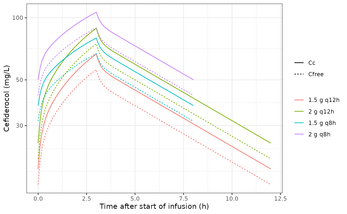
Typical-value steady-state total (solid) and free (dashed) cefiderocol over the final dosing interval for each label regimen.
PKNCA against the closed form
nca_conc_tv <- sim_tv %>%
  dplyr::filter(!is.na(Cc)) %>%
  dplyr::select(id, regimen, time, Cc)
nca_dose_tv <- ev_tv %>%
  dplyr::filter(evid == 1) %>%
  dplyr::select(id, regimen, time, amt)
int_tv <- regimens %>%
  dplyr::transmute(
    regimen, start = TEND - tau, end = TEND,
    auclast = TRUE, cmax = TRUE, cmin = TRUE
  )
nca_tv <- as.data.frame(PKNCA::pk.nca(PKNCA::PKNCAdata(
  PKNCA::PKNCAconc(nca_conc_tv, Cc ~ time | regimen + id,
                   concu = "mg/L", timeu = "h"),
  PKNCA::PKNCAdose(nca_dose_tv, amt ~ time | regimen + id,
                   doseu = "mg", duration = DUR),
  intervals = int_tv
)))

tv_chk <- nca_tv %>%
  dplyr::select(regimen, PPTESTCD, PPORRES) %>%
  tidyr::pivot_wider(names_from = PPTESTCD, values_from = PPORRES) %>%
  dplyr::left_join(regimens, by = "regimen") %>%
  dplyr::mutate(
    auc_daily = auclast * 24 / tau,
    closed_form = daily_dose / th[["lcl"]],
    pct = 100 * (auc_daily - closed_form) / closed_form
  )
tv_chk %>%
  dplyr::transmute(
    regimen, band, cmax, cmin, auc_daily, closed_form, pct
  ) %>%
  dplyr::rename(
    "Regimen" = regimen, "Effluent band" = band,
    "Cmax (mg/L)" = cmax, "Ctrough (mg/L)" = cmin,
    "AUCdaily, PKNCA (mg*h/L)" = auc_daily,
    "Daily dose / CL (mg*h/L)" = closed_form, "% diff" = pct
  ) %>%
knitr::kable(digits = 2, caption = "Typical patient at steady state.")| Regimen | Effluent band | Cmax (mg/L) | Ctrough (mg/L) | AUCdaily, PKNCA (mg*h/L) | Daily dose / CL (mg*h/L) | % diff |
|---|---|---|---|---|---|---|
| 1.5 g q12h | <= 2 L/h | 66.70 | 18.50 | 909.07 | 909.09 | 0 |
| 2 g q12h | 2.1-3 L/h | 88.93 | 24.67 | 1212.09 | 1212.12 | 0 |
| 1.5 g q8h | 3.1-4 L/h | 79.77 | 37.56 | 1363.60 | 1363.64 | 0 |
| 2 g q8h | >= 4.1 L/h | 106.36 | 50.08 | 1818.14 | 1818.18 | 0 |
Mean or median as the typical value
Table 2 reports each parameter’s mean +/- SD and median. The paper’s own exposure summary, the pooled AUCdaily of 1444 +/- 423 mgh/L (Results) with a median of about 1430 and an interquartile range of about 1290-1720 mgh/L (digitised from the CRRT box of Figure 2), depends only on the clearance distribution and the label dose of each patient’s effluent band, because AUCdaily is the daily dose divided by clearance. With a lognormal clearance it can therefore be computed exactly, without simulation, for either choice of typical value. The patients are weighted by the Table 1 effluent bands.
w  <- regimens$n_paper / sum(regimens$n_paper)
DD <- regimens$daily_dose
om_cl <- ui$omega["etalcl", "etalcl"]

aucDist <- function(tvcl) {
  mu <- log(tvcl)
  cdf <- function(a) sum(w * (1 - plnorm(DD / a, mu, sqrt(om_cl))))
  q <- vapply(
    c(0.25, 0.5, 0.75),
    function(p) uniroot(function(a) cdf(a) - p, c(10, 1e5))$root,
    numeric(1)
  )
  c(mean = sum(w * DD) * exp(-mu + om_cl / 2), q1 = q[1], median = q[2], q3 = q[3])
}
published <- c(mean = 1444, q1 = 1290, median = 1430, q3 = 1720)
mm <- rbind(
  Published = published,
  `Median column (CL 3.3)` = aucDist(3.3),
  `Mean column (CL 3.5)` = aucDist(3.5)
)
knitr::kable(
  as.data.frame(mm) %>%
    dplyr::rename(
      "Mean AUCdaily" = mean, "Q1" = q1, "Median" = median, "Q3" = q3
    ),
  digits = 0,
  caption = paste(
    "Pooled AUCdaily (mg*h/L) under label dosing. Published mean from the",
    "Results; quartiles digitised from Figure 2."
  )
)| Mean AUCdaily | Q1 | Median | Q3 | |
|---|---|---|---|---|
| Published | 1444 | 1290 | 1430 | 1720 |
| Median column (CL 3.3) | 1466 | 997 | 1334 | 1786 |
| Mean column (CL 3.5) | 1382 | 940 | 1258 | 1684 |
stopifnot(
  # Deterministic. The median column gives +1.5% on the mean and -6.7% on the
  # median; the mean column gives -4.3% and -12%.
  abs(mm[2, "mean"] / 1444 - 1) < 0.03,
  abs(mm[2, "median"] / 1430 - 1) < abs(mm[3, "median"] / 1430 - 1)
)
The median column lands closer on both the mean and the median, and it is also the reading under which Table 2 is internally consistent: a lognormal with the printed median and the SD-derived variance has a mean of 3.58 L/h for CL, 3.85 1/h for k12 and 2.12 1/h for k21, against the printed means of 3.5, 3.9 and 2.2. The model therefore encodes the medians.
The modelled interquartile range is wider than the published one (Q1 997 against about 1290). The study dosed by effluent band, and effluent flow was correlated with clearance (Supplementary Figure S1), so the bands partly cancelled the between-patient spread in clearance. The final model carries no effluent covariate, so the simulation assigns doses independently of clearance, and that link is lost.
Stochastic cohort under label dosing
A virtual cohort of 280 patients is split across the four effluent bands in the Table 1 proportions (20 per study patient: 20, 80, 140 and 40), so no arm exceeds 200.
rxode2::rxSetSeed(20241015)
n_arm <- regimens$n_paper * 20
reg_id <- rep(seq_len(nrow(regimens)), n_arm)
ev_vpc <- mkEvents(seq_along(reg_id), reg_id, grid = 0.25)
sim <- as.data.frame(rxode2::rxSolve(
  ui, events = ev_vpc, keep = "regimen", returnType = "data.frame"
))
sim <- dplyr::left_join(sim, regimens[, c("regimen", "tau")], by = "regimen")
sim %>%
  dplyr::mutate(
    tad = time - (TEND - tau),
    regimen = factor(regimen, levels = regimens$regimen)
  ) %>%
  dplyr::group_by(regimen, tad) %>%
  dplyr::summarise(
    lo = quantile(Cc, 0.05), med = median(Cc), hi = quantile(Cc, 0.95),
    .groups = "drop"
  ) %>%
  ggplot(aes(tad, med)) +
  geom_ribbon(aes(ymin = lo, ymax = hi), alpha = 0.25) +
  geom_line() +
  facet_wrap(~regimen) +
  scale_y_log10() +
  labs(x = "Time after start of infusion (h)", y = "Total cefiderocol (mg/L)") +
  theme_bw()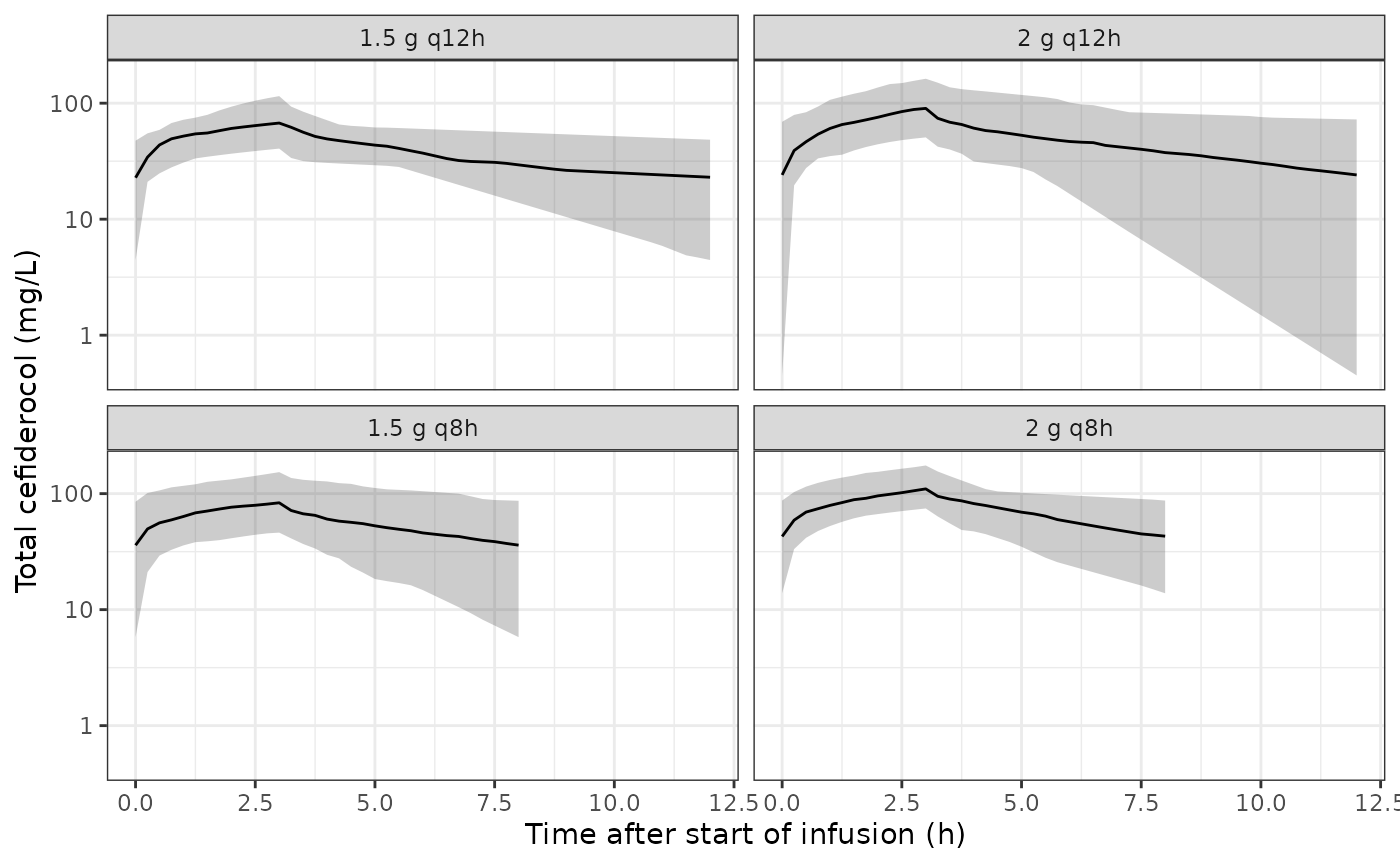
Steady-state total cefiderocol over the final dosing interval by label regimen: median and 5th-95th percentiles of the virtual cohort.
PKNCA: pooled AUCdaily
nca_conc <- sim %>%
  dplyr::filter(!is.na(Cc)) %>%
  dplyr::select(id, regimen, time, Cc)
nca_dose <- ev_vpc %>%
  dplyr::filter(evid == 1) %>%
  dplyr::select(id, regimen, time, amt)
nca_res <- as.data.frame(PKNCA::pk.nca(PKNCA::PKNCAdata(
  PKNCA::PKNCAconc(nca_conc, Cc ~ time | regimen + id,
                   concu = "mg/L", timeu = "h"),
  PKNCA::PKNCAdose(nca_dose, amt ~ time | regimen + id,
                   doseu = "mg", duration = DUR),
  intervals = int_tv
)))

auc_daily <- nca_res %>%
  dplyr::filter(PPTESTCD == "auclast") %>%
  dplyr::left_join(regimens[, c("regimen", "tau")], by = "regimen") %>%
  dplyr::transmute(
    id, regimen, PPTESTCD = "auclast", PPORRES = PPORRES * 24 / tau
  )
stopifnot(nrow(auc_daily) == sum(n_arm))

cmp <- nlmixr2lib::ncaComparisonTable(
  auc_daily, data.frame(auclast = 1430),
  params = "auclast",
  units = c(auclast = "mg*h/L, AUCdaily = AUCtau x 24 / tau")
)
knitr::kable(
  cmp,
  caption = paste(
    "Pooled median AUCdaily against the CRRT median digitised from Fouad 2024",
    "Figure 2.", attr(cmp, "footnote")
  )
)| NCA parameter | Reference | Simulated | % diff |
|---|---|---|---|
| AUClast (mg*h/L, AUCdaily = AUCtau x 24 / tau) | 1430 | 1330 | -7.0% |
sprintf(
  "simulated pooled AUCdaily: mean %.0f, SD %.0f, median %.0f (published mean 1444 +/- 423)",
  mean(auc_daily$PPORRES), sd(auc_daily$PPORRES), median(auc_daily$PPORRES)
)
#> [1] "simulated pooled AUCdaily: mean 1450, SD 658, median 1330 (published mean 1444 +/- 423)"
stopifnot(
  # Exact model value is 1334 (deterministic chunk above); a mis-transcribed
  # clearance or dose moves it by tens of percent. 280 patients put the
  # Monte Carlo SE of the median near 3%.
  abs(median(auc_daily$PPORRES) / 1430 - 1) < 0.2
)
pub_box <- data.frame(
  source = "Published (n = 14)", ymin = 644, lower = 1290, middle = 1430,
  upper = 1720, ymax = 2156
)
sim_box <- auc_daily %>%
  dplyr::summarise(
    ymin = min(PPORRES), lower = quantile(PPORRES, 0.25),
    middle = median(PPORRES), upper = quantile(PPORRES, 0.75),
    ymax = max(PPORRES)
  ) %>%
  dplyr::mutate(source = "Simulated (n = 280)")
ggplot(rbind(pub_box, sim_box[, names(pub_box)]), aes(x = source)) +
  geom_boxplot(
    aes(ymin = ymin, lower = lower, middle = middle, upper = upper, ymax = ymax,
        fill = source),
    stat = "identity", width = 0.5
  ) +
  scale_fill_manual(values = c("grey70", "steelblue"), guide = "none") +
  labs(x = NULL, y = "AUCdaily (mg*h/L)") +
  theme_bw()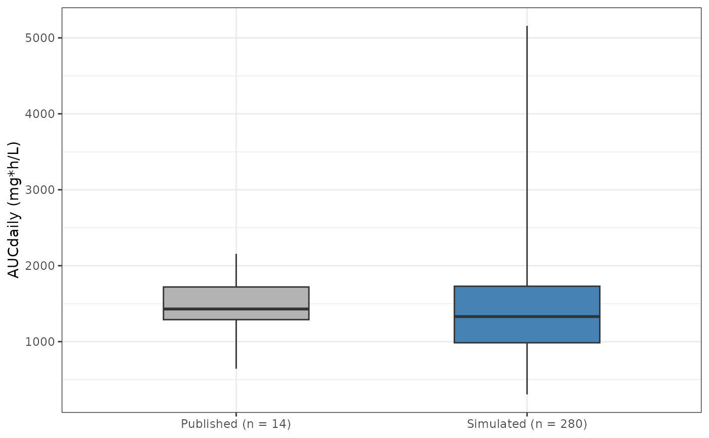
Replicates the CRRT box of Fouad 2024 Figure 2: AUCdaily under label dosing. Box = interquartile range, whiskers = minimum and maximum. The grey box is the published one (digitised); the simulated box pools the four effluent bands.
Free time above the MIC
Table 3 gives each patient’s %fT > MIC under the label dose for their effluent band. Below, the share of patients reaching 100% and at least 75% fT > MIC (the clinical-success target) is compared with the share of the virtual cohort.
mics <- c(0.5, 1, 2, 4, 8, 16, 32)
sim_last <- dplyr::filter(sim, time > TEND - tau)
ft_mat <- vapply(
  mics,
  function(m) 100 * tapply(sim_last$Cfree > m, sim_last$id, mean),
  numeric(length(unique(sim_last$id)))
)

# Fouad 2024 Table 3, patients 1-14; MICs 0.5-8 mg/L are 100% for everyone.
ft_pub <- cbind(
  matrix(100, nrow = 14, ncol = 5),
  c(100, 100, 100, 100, 100, 100, 100, 82, 100, 100, 100, 100, 100, 100),
  c(94, 100, 92, 75, 100, 86, 94, 0, 49, 100, 100, 99, 100, 6)
)
stopifnot(nrow(ft_mat) == sum(n_arm), ncol(ft_mat) == length(mics))

ftmic <- data.frame(
  MIC = mics,
  pub100 = 100 * colMeans(ft_pub >= 100),
  sim100 = 100 * colMeans(ft_mat >= 100),
  pub75 = 100 * colMeans(ft_pub >= 75),
  sim75 = 100 * colMeans(ft_mat >= 75)
)
ftmic %>%
  dplyr::rename(
    "MIC (mg/L)" = MIC,
    "100% fT>MIC, published (%)" = pub100,
    "100% fT>MIC, simulated (%)" = sim100,
    ">= 75% fT>MIC, published (%)" = pub75,
    ">= 75% fT>MIC, simulated (%)" = sim75
  ) %>%
knitr::kable(digits = 1, caption = "Share of patients reaching the target.")| MIC (mg/L) | 100% fT>MIC, published (%) | 100% fT>MIC, simulated (%) | >= 75% fT>MIC, published (%) | >= 75% fT>MIC, simulated (%) |
|---|---|---|---|---|
| 0.5 | 100.0 | 98.2 | 100.0 | 99.6 |
| 1.0 | 100.0 | 97.1 | 100.0 | 98.9 |
| 2.0 | 100.0 | 95.0 | 100.0 | 98.9 |
| 4.0 | 100.0 | 92.1 | 100.0 | 97.9 |
| 8.0 | 100.0 | 86.8 | 100.0 | 93.2 |
| 16.0 | 92.9 | 75.0 | 100.0 | 86.8 |
| 32.0 | 35.7 | 41.1 | 78.6 | 57.5 |
stopifnot(
  # The paper's headline claim is that every patient reaches 100% fT > MIC up
  # to 8 mg/L under label dosing. At the 4 mg/L susceptible breakpoint the
  # virtual cohort reaches the 75% target in about 98% of patients and 100%
  # fT > MIC in about 92%; these bounds are set well inside those values
  # because they are shares of a random cohort's tail.
  ftmic$sim75[ftmic$MIC == 4] > 90,
  ftmic$sim100[ftmic$MIC == 4] > 80
)
All 14 study patients reached 100% fT > MIC up to 8 mg/L. The virtual cohort reaches the clinical 75% target in at least 93% of patients up to 8 mg/L, but 100% fT > MIC in fewer of them (about 92% at 4 mg/L and 87% at 8 mg/L). At 32 mg/L the share reaching 100% is close to the paper’s (5 of 14), while the share reaching 75% is lower (11 of 14 in the paper). The shortfall sits in the low tail of the trough distribution, which is set by the wide spread of k21 and Vc (CVs of 100% and 79%) and by the clearance-dose link discussed above. A lognormal with independent etas puts more weight in that tail than the 14 individual posterior estimates did, so the model is conservative for target attainment at the upper MICs.
Individual clearances recovered from Table S3
Table S3 gives, for each of the nine patients dosed off-label, the AUCdaily of both the actual and the label regimen. Since AUCdaily is daily dose divided by the individual Bayesian clearance, both rows return the same clearance, which checks the transcription and places nine of the 14 individual clearances against the model’s distribution.
s3 <- data.frame(
  patient = c(2, 3, 4, 5, 7, 8, 9, 13, 14),
  effluent = c(2.08, 2.14, 3.67, 3.41, 4.77, 3.34, 5.06, 3.02, 3.15),
  dd_actual = c(3000, 4000, 8000, 8000, 8000, 6000, 8000, 8000, 4000),
  auc_actual = c(1617, 1966, 2494, 2482, 2086, 859, 1376, 1628, 1182),
  dd_label = c(4000, 3000, 4500, 4500, 6000, 4500, 6000, 4000, 4500),
  auc_label = c(2156, 1474, 1403, 1396, 1565, 644, 1032, 814, 1329)
)
s3 <- s3 %>%
  dplyr::mutate(
    cl_actual = dd_actual / auc_actual,
    cl_label = dd_label / auc_label,
    pct_model = 100 * plnorm(cl_actual, log(th[["lcl"]]), sqrt(om_cl))
  )
s3 %>%
  dplyr::rename(
    "Patient" = patient, "Effluent (L/h)" = effluent,
    "CL from actual regimen (L/h)" = cl_actual,
    "CL from label regimen (L/h)" = cl_label,
    "Percentile of model CL" = pct_model
  ) %>%
  dplyr::select(-dd_actual, -auc_actual, -dd_label, -auc_label) %>%
knitr::kable(digits = 2)| Patient | Effluent (L/h) | CL from actual regimen (L/h) | CL from label regimen (L/h) | Percentile of model CL |
|---|---|---|---|---|
| 2 | 2.08 | 1.86 | 1.86 | 7.52 |
| 3 | 2.14 | 2.03 | 2.04 | 11.36 |
| 4 | 3.67 | 3.21 | 3.21 | 47.18 |
| 5 | 3.41 | 3.22 | 3.22 | 47.66 |
| 7 | 4.77 | 3.84 | 3.83 | 64.62 |
| 8 | 3.34 | 6.98 | 6.99 | 96.94 |
| 9 | 5.06 | 5.81 | 5.81 | 92.13 |
| 13 | 3.02 | 4.91 | 4.91 | 83.99 |
| 14 | 3.15 | 3.38 | 3.39 | 52.50 |
stopifnot(
  # AUCs are printed to the nearest mg*h/L, so the two clearances agree to
  # rounding (realised max 0.06%).
  max(abs(s3$cl_actual / s3$cl_label - 1)) < 0.005
)
All nine fall between the 7th and 97th percentiles of the model’s clearance distribution. Clearance rises with effluent flow among them (patients 2 and 3 at about 2.1 L/h have the two lowest clearances), which is the correlation the authors report in Supplementary Figure S1 but did not retain in the model.
Assumptions and deviations
-
Median column as the typical value. Table 2 gives
mean +/- SD and median. The medians are encoded as lognormal medians and
the SDs become lognormal variances via
omega^2 = log(1 + (SD/mean)^2). The choice is supported by the closed-form AUCdaily comparison above and by the internal consistency of Table 2 under a lognormal; for Vc the lognormal mean (9.4 L) is below the printed mean (10.7 L), reflecting a right tail heavier than lognormal in the NPAG density. - Independent etas. No covariance or correlation matrix of the nonparametric joint density is published, so the four etas are independent. The shape of the NPAG density, including any multimodality, cannot be recovered from Table 2.
-
Residual error. The Pmetrics assay polynomial
0.006 + 0.06 * Cis multiplied by the published fitted gamma of 1.6 and encoded ascombined1(), since Pmetrics sums the additive and proportional parts linearly. Pmetrics evaluates the polynomial at the observed concentration; nlmixr2 evaluates it at the prediction. -
No covariates on disposition. Body weight, effluent
flow and transmembrane clearance correlated with individual clearance
but did not improve AIC and are not in the final model; they are
documented in
covariatesDataExcluded. Simulations by effluent band therefore draw clearance independently of the band, which widens the modelled AUCdaily distribution relative to the study’s. -
Fraction unbound.
Cfree = FU * Ccuses the measured per-patient fraction unbound as a covariate. Per-patient values are not published; the simulations use the cohort mean 0.84. Typical non-critically ill binding is 40-60%, so FU around 0.5 is the appropriate input outside this population. - Figure 2 values (median 1430, quartiles 1290 and 1720, whiskers 644 and 2156 mg*h/L) were digitised by the maintainers from the published figure; the whiskers coincide with the Table S3 label-regimen extremes (patient 8: 644, patient 2: 2156), which anchors the digitisation.
- Population. All patients were on CVVHDF with effluent flows of 2.08-5.1 L/h. The model is not informed by other CRRT modalities, by intermittent dialysis, or by effluent flows outside that range, and residual renal function was present in some patients but not modelled.
Errata and provenance notes
- Table 2 prints the CL SD as 1.46 L/h; the Abstract rounds it to 1.5. The Table 2 value is used.
- No erratum or correction to this article was found on Europe PMC (checked 2026-10-30).
- The same group’s sibling model in people with cystic fibrosis is
Koenig_2025_cefiderocol, which has the same CL / Vc / k12 / k21 parameterisation. The CRRT clearance here (3.3 L/h) is lower than that cohort’s (5.66 L/h, normal-to-augmented renal function) and the fraction unbound is higher (0.84 against 0.52).