Bintrafusp alfa and pembrolizumab tumor dynamics in BTC and NSCLC (Milenkovic-Grisic 2024)
Source:vignettes/articles/MilenkovicGrisic_2024_tumor_dynamics.Rmd
MilenkovicGrisic_2024_tumor_dynamics.RmdModel and source
- Citation: Milenkovic-Grisic A-M, Terranova N, Mould DR, Vugmeyster Y, Mrowiec T, Machl A, Girard P, Venkatakrishnan K, Khandelwal A. Tumor growth inhibition modeling in patients with second line biliary tract cancer and first line non-small cell lung cancer based on bintrafusp alfa trials. CPT Pharmacometrics Syst Pharmacol. 2024;13(1):143-153. doi:10.1002/psp4.13068
- Article: https://doi.org/10.1002/psp4.13068 (open access; PubMed Central PMC10787199)
- Supplement: Data S1 (covariate lists, Tables S1-S4, Figures S1-S5)
Milenkovic-Grisic 2024 fits one empirical tumor-size model per drug and indication from two trials of bintrafusp alfa (BA), a bifunctional fusion protein targeting TGF-beta and PD-L1:
| Model file | Trial | Treatment | Covariates |
|---|---|---|---|
MilenkovicGrisic_2024_bintrafuspAlfa_btc |
INTR@PID BTC 047 (NCT03833661), phase II | BA 1200 mg IV q2w, second-line biliary tract cancer | 10 covariate effects + BA exposure (AUC) |
MilenkovicGrisic_2024_bintrafuspAlfa_nsclc |
INTR@PID Lung 037 (NCT03631706), phase III | BA 1200 mg IV q2w, first-line PD-L1-high NSCLC | CRP on BTS, lymphocyte % on kg |
MilenkovicGrisic_2024_pembrolizumab_nsclc |
INTR@PID Lung 037 (NCT03631706), phase III | pembrolizumab 200 mg IV q3w, first-line PD-L1-high NSCLC | none |
The three models were estimated separately, so they are packaged as three files. All share the structure of Eq 1 of the paper, with time t in weeks from the first dose:
and the log-transform-both-sides residual error of Eq 2,
.
In the package BTS is rbase, ks
is kse and kg is p; the output is
tumor_size (mm).
Population
pops <- lapply(
  c("MilenkovicGrisic_2024_bintrafuspAlfa_btc",
    "MilenkovicGrisic_2024_bintrafuspAlfa_nsclc",
    "MilenkovicGrisic_2024_pembrolizumab_nsclc"),
  function(nm) {
    p <- rxode2::rxode(readModelDb(nm))$population
    tibble::tibble(
      Model = nm, N = p$n_subjects, Age = p$age_range, Weight = p$weight_range,
      `Female (%)` = p$sex_female_pct
    )
  }
)
#> ℹ parameter labels from comments will be replaced by 'label()'
#> ℹ parameter labels from comments will be replaced by 'label()'
#> ℹ parameter labels from comments will be replaced by 'label()'
knitr::kable(dplyr::bind_rows(pops))| Model | N | Age | Weight | Female (%) |
|---|---|---|---|---|
| MilenkovicGrisic_2024_bintrafuspAlfa_btc | 143 | median 65 years (range 39-83) | median 65 kg (range 38-100) | 40.6 |
| MilenkovicGrisic_2024_bintrafuspAlfa_nsclc | 139 | median 67 years (range 42-90) | median 66.5 kg (range 35.0-104.3) | 20.1 |
| MilenkovicGrisic_2024_pembrolizumab_nsclc | 143 | median 67 years (range 36-88) | median 66.9 kg (range 40.0-141.5) | 22.4 |
Demographics are from the Results text of each tumor-dynamics subsection (2L BTC: 143 of 157 treated patients with evaluable PK and tumor-size data; 1L NSCLC: 139 of 152 BA-treated and 143 of 152 pembrolizumab-treated patients). Tumor size is the RECIST 1.1 sum of longest diameters of the target lesions, in mm. The paper reports no distribution for any of the retained covariates (CRP, AST, minor allele frequency, time since diagnosis, lymphocyte percentage, IDH1, blood TMB, Asian race).
Source trace
| Quantity | Value(s) | Source |
|---|---|---|
| Structure TS(t) = BTS exp(-ks t) + kg t | – | Eq 1 |
| Residual error, log-transform both sides, additive | – | Eq 2 |
| BTC: BTS, ks, kg | 51.3 mm, 0.0159 /week, 0.624 mm/week | Table 1; Results text |
| BTC: AUC effect on ks | 0.339 | Table 1 |
| BTC: MAF, time since diagnosis, AST, CRP, Asian race on BTS | 0.106, -0.151, 0.189, 0.0777, -0.2 | Table 1 |
| BTC: IDH1 on ks | 2.13 | Table 1 |
| BTC: MAF, IDH1, CRP, blood TMB on kg | 0.262, 1.17, 0.152, 0.629 | Table 1 |
| BTC: IIV BTS / ks / kg (%CV); correlations | 50 / 103.4 / 72.7; -0.362, 0.465, -0.845 | Table 1 |
| BTC: residual error (%CV) | 15.6 | Table 1 |
| NSCLC BA: BTS, ks, kg | 81.1 mm, 0.0368 /week, 0.728 mm/week | Table 2; Results text |
| NSCLC BA: CRP on BTS, lymphocyte % on kg | 0.125, -0.623 | Table 2 |
| NSCLC BA: IIV (%CV); correlations | 55.4 / 62.8 / 122.9; -0.0411, 0.423, -0.0639 | Table 2 |
| NSCLC BA: residual error (%CV) | 12.8 | Table 2 |
| NSCLC pembrolizumab: BTS, ks, kg | 80.4 mm, 0.0307 /week, 0.643 mm/week | Table 2; Results text |
| NSCLC pembrolizumab: IIV (%CV); correlations | 55.5 / 70.1 / 92.7; -0.0228, 0.288, -0.0834 | Table 2 |
| NSCLC pembrolizumab: residual error (%CV) | 11.3 | Table 2 |
| Categorical covariate reference levels | non-Asian, no IDH1 mutation, blood TMB < 50th percentile | Figure 3 caption |
| Categorical effect form (1 + theta) | – | reproduced from Figure 3e-g (below) |
| Continuous covariate form and reference values; AUC normalisation | – | not reported; maintainers’ assumptions (see Errata) |
IIV conversion
Tables 1 and 2 report the IIV as %CV of log-normal random effects. The model files store variances and covariances . Back-transforming recovers the published numbers.
iivTable <- function(nm, cvPub, corPub) {
  om <- rxode2::rxode(readModelDb(nm))$omega
  om <- om[c("etalrbase", "etalkse", "etalp"), c("etalrbase", "etalkse", "etalp")]
  cv <- 100 * sqrt(exp(diag(om)) - 1)
  cr <- stats::cov2cor(om)
  tibble::tibble(
    Model = nm,
    Quantity = c("CV BTS", "CV ks", "CV kg", "Corr(BTS,ks)", "Corr(BTS,kg)", "Corr(ks,kg)"),
    Published = c(cvPub, corPub),
    Packaged = c(cv, cr[1, 2], cr[1, 3], cr[2, 3])
  )
}
iiv <- dplyr::bind_rows(
  iivTable("MilenkovicGrisic_2024_bintrafuspAlfa_btc", c(50, 103.4, 72.7), c(-0.362, 0.465, -0.845)),
  iivTable("MilenkovicGrisic_2024_bintrafuspAlfa_nsclc", c(55.4, 62.8, 122.9), c(-0.0411, 0.423, -0.0639)),
  iivTable("MilenkovicGrisic_2024_pembrolizumab_nsclc", c(55.5, 70.1, 92.7), c(-0.0228, 0.288, -0.0834))
)
#> ℹ parameter labels from comments will be replaced by 'label()'
#> ℹ parameter labels from comments will be replaced by 'label()'
#> ℹ parameter labels from comments will be replaced by 'label()'
knitr::kable(iiv, digits = 4)| Model | Quantity | Published | Packaged |
|---|---|---|---|
| MilenkovicGrisic_2024_bintrafuspAlfa_btc | CV BTS | 50.0000 | 49.9946 |
| MilenkovicGrisic_2024_bintrafuspAlfa_btc | CV ks | 103.4000 | 103.3959 |
| MilenkovicGrisic_2024_bintrafuspAlfa_btc | CV kg | 72.7000 | 72.6994 |
| MilenkovicGrisic_2024_bintrafuspAlfa_btc | Corr(BTS,ks) | -0.3620 | -0.3620 |
| MilenkovicGrisic_2024_bintrafuspAlfa_btc | Corr(BTS,kg) | 0.4650 | 0.4651 |
| MilenkovicGrisic_2024_bintrafuspAlfa_btc | Corr(ks,kg) | -0.8450 | -0.8451 |
| MilenkovicGrisic_2024_bintrafuspAlfa_nsclc | CV BTS | 55.4000 | 55.4035 |
| MilenkovicGrisic_2024_bintrafuspAlfa_nsclc | CV ks | 62.8000 | 62.8052 |
| MilenkovicGrisic_2024_bintrafuspAlfa_nsclc | CV kg | 122.9000 | 122.9042 |
| MilenkovicGrisic_2024_bintrafuspAlfa_nsclc | Corr(BTS,ks) | -0.0411 | -0.0411 |
| MilenkovicGrisic_2024_bintrafuspAlfa_nsclc | Corr(BTS,kg) | 0.4230 | 0.4230 |
| MilenkovicGrisic_2024_bintrafuspAlfa_nsclc | Corr(ks,kg) | -0.0639 | -0.0639 |
| MilenkovicGrisic_2024_pembrolizumab_nsclc | CV BTS | 55.5000 | 55.4978 |
| MilenkovicGrisic_2024_pembrolizumab_nsclc | CV ks | 70.1000 | 70.0983 |
| MilenkovicGrisic_2024_pembrolizumab_nsclc | CV kg | 92.7000 | 92.6984 |
| MilenkovicGrisic_2024_pembrolizumab_nsclc | Corr(BTS,ks) | -0.0228 | -0.0228 |
| MilenkovicGrisic_2024_pembrolizumab_nsclc | Corr(BTS,kg) | 0.2880 | 0.2879 |
| MilenkovicGrisic_2024_pembrolizumab_nsclc | Corr(ks,kg) | -0.0834 | -0.0834 |
Typical-value profiles
All covariates at the reference profile used by the model files:
minor allele frequency 1 percent, 365 days since diagnosis, AST 30 U/L,
CRP 10 mg/L, lymphocytes 20 percent of leukocytes, non-Asian, IDH1 wild
type, blood TMB below the median and the median BA exposure
(AUC_BINTRAFUSP_REL = 1).
refCov <- data.frame(
  CTDNA_VAF = 1, T_DIAG_CANCER = 365, AST = 30, CRP = 10, RACE_ASIAN = 0,
  TUM_IDH1_MUT = 0, TUM_MUTATIONAL_BURDEN_BLOOD_HIGH = 0, AUC_BINTRAFUSP_REL = 1, LYMPH_PCT = 20
)
models <- c(
  "BA, 2L BTC" = "MilenkovicGrisic_2024_bintrafuspAlfa_btc",
  "BA, 1L NSCLC" = "MilenkovicGrisic_2024_bintrafuspAlfa_nsclc",
  "Pembrolizumab, 1L NSCLC" = "MilenkovicGrisic_2024_pembrolizumab_nsclc"
)
tgrid <- seq(0, 65, by = 0.25)

solveTypical <- function(nm, cov = refCov, mod = NULL) {
  if (is.null(mod)) mod <- rxode2::zeroRe(rxode2::rxode(readModelDb(nm)))
  ev <- data.frame(id = 1L, time = tgrid) |> dplyr::cross_join(cov)
  as.data.frame(rxode2::rxSolve(mod, ev))
}
typ <- dplyr::bind_rows(lapply(names(models), function(a) {
  solveTypical(models[[a]]) |> dplyr::mutate(Arm = a)
}))
#> ℹ parameter labels from comments will be replaced by 'label()'
#> ℹ omega/sigma items treated as zero: 'etalrbase', 'etalkse', 'etalp'
#> ℹ parameter labels from comments will be replaced by 'label()'
#> ℹ omega/sigma items treated as zero: 'etalrbase', 'etalkse', 'etalp'
#> ℹ parameter labels from comments will be replaced by 'label()'
#> ℹ omega/sigma items treated as zero: 'etalrbase', 'etalkse', 'etalp'

# Structural identity: the solved profile equals Eq 1 evaluated with the same
# individual parameters (pure floating-point difference).
stopifnot(max(abs(typ$tumor_size - (typ$rbase * exp(-typ$kse * typ$time) + typ$p * typ$time))) < 1e-8)

# At the reference profile every covariate multiplier is exactly 1, so the
# typical parameters are the published Table 1 / Table 2 values.
anchors <- typ |> dplyr::filter(time == 0) |> dplyr::select(Arm, BTS = rbase, ks = kse, kg = p)
knitr::kable(anchors, digits = 4)| Arm | BTS | ks | kg |
|---|---|---|---|
| BA, 2L BTC | 51.3 | 0.0159 | 0.624 |
| BA, 1L NSCLC | 81.1 | 0.0368 | 0.728 |
| Pembrolizumab, 1L NSCLC | 80.4 | 0.0307 | 0.643 |
stopifnot(
  isTRUE(all.equal(anchors$BTS, c(51.3, 81.1, 80.4), tolerance = 1e-8)),
  isTRUE(all.equal(anchors$ks, c(0.0159, 0.0368, 0.0307), tolerance = 1e-8)),
  isTRUE(all.equal(anchors$kg, c(0.624, 0.728, 0.643), tolerance = 1e-8))
)

# Time and depth of the nadir: dTS/dt = 0 at t* = log(BTS * ks / kg) / ks.
nadir <- typ |>
  dplyr::group_by(Arm) |>
  dplyr::summarise(
    t_grid = time[which.min(tumor_size)], ts_min = min(tumor_size),
    t_closed = log(rbase[1] * kse[1] / p[1]) / kse[1], .groups = "drop"
  )
nadir |>
  dplyr::rename(
    "Nadir time, grid (weeks)" = t_grid, "Nadir size (mm)" = ts_min,
    "Nadir time, closed form (weeks)" = t_closed
  ) |>
knitr::kable(digits = 2)| Arm | Nadir time, grid (weeks) | Nadir size (mm) | Nadir time, closed form (weeks) |
|---|---|---|---|
| BA, 1L NSCLC | 38.25 | 47.69 | 38.34 |
| BA, 2L BTC | 16.75 | 49.76 | 16.85 |
| Pembrolizumab, 1L NSCLC | 43.75 | 49.12 | 43.82 |
ggplot(typ, aes(time, tumor_size, colour = Arm)) +
  geom_line(linewidth = 1) +
  labs(x = "Time since first dose (weeks)", y = "Tumor size (mm)", colour = NULL) +
  theme_bw() +
  theme(legend.position = "bottom")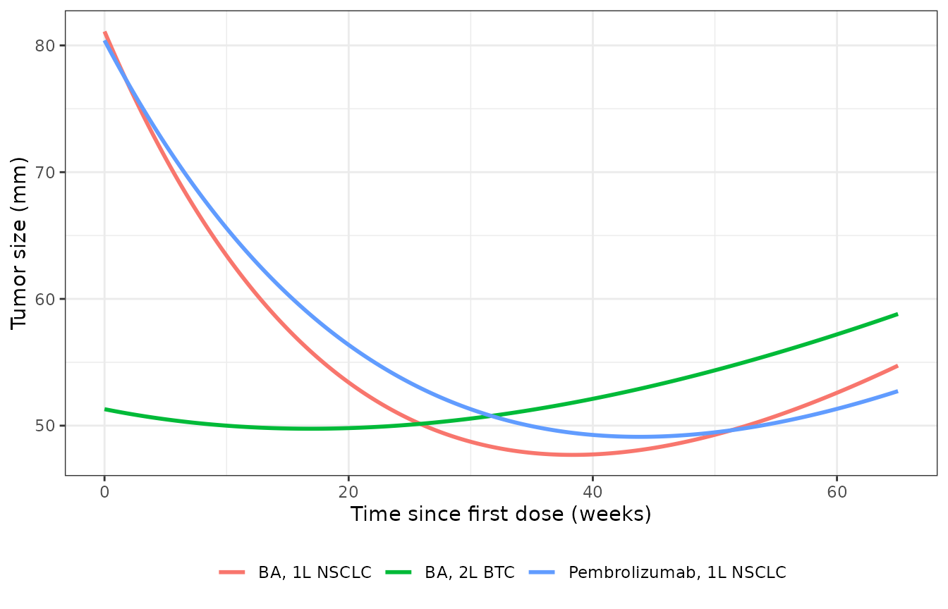
Typical-value tumor-size profiles at the reference covariate profile for the three models.
Replicating Figure 3 (covariate effects)
Figure 3 shows typical-patient profiles over 65 weeks for each
covariate. Its “median” (purple) curves do not start at the typical BTS
of Tables 1 and 2: the BTC panels start near 68 mm (typical 51.3 mm) and
the NSCLC panels near 88 mm (typical 81.1 mm). The tabulated typical
values therefore belong to an unreported reference covariate profile,
not to the cohort median. To compare shapes, the BTC model is
re-anchored here at the Figure 3 starting value
(lrbase = log(68)) with all other parameters as packaged;
the values in the check table were read off Figure 3 by the
maintainers.
btcMod <- rxode2::zeroRe(rxode2::rxode(readModelDb("MilenkovicGrisic_2024_bintrafuspAlfa_btc")))
#> ℹ parameter labels from comments will be replaced by 'label()'
btcFig3 <- btcMod |> rxode2::ini(lrbase = log(68))
#> ℹ change initial estimate of `lrbase` to `4.21950770517611`

panels <- list(
  "Reference (non-Asian, IDH1 wild type, TMB < median)" = refCov,
  "Asian race (Figure 3e)" = dplyr::mutate(refCov, RACE_ASIAN = 1),
  "IDH1 mutation (Figure 3f)" = dplyr::mutate(refCov, TUM_IDH1_MUT = 1),
  "Blood TMB >= median (Figure 3g)" = dplyr::mutate(refCov, TUM_MUTATIONAL_BURDEN_BLOOD_HIGH = 1)
)
fig3 <- dplyr::bind_rows(lapply(names(panels), function(nm) {
  solveTypical(NULL, panels[[nm]], btcFig3) |> dplyr::mutate(Profile = nm)
}))
#> ℹ omega/sigma items treated as zero: 'etalrbase', 'etalkse', 'etalp'
#> ℹ omega/sigma items treated as zero: 'etalrbase', 'etalkse', 'etalp'
#> ℹ omega/sigma items treated as zero: 'etalrbase', 'etalkse', 'etalp'
#> ℹ omega/sigma items treated as zero: 'etalrbase', 'etalkse', 'etalp'
at <- function(prof, t) fig3$tumor_size[fig3$Profile == prof & abs(fig3$time - t) < 1e-9]

fig3chk <- tibble::tribble(
  ~Check, ~Figure3, ~Model,
  "Reference, minimum (mm)", 61, min(fig3$tumor_size[fig3$Profile == names(panels)[1]]),
  "Reference, week 65 (mm)", 64, at(names(panels)[1], 65),
  "Asian, week 0 (mm)", 54, at(names(panels)[2], 0),
  "IDH1 mutant, week 20 (mm)", 52, at(names(panels)[3], 20),
  "IDH1 mutant, week 65 (mm)", 91, at(names(panels)[3], 65),
  "Blood TMB high, week 65 (mm)", 90, at(names(panels)[4], 65)
)
fig3chk |>
  dplyr::rename("Figure 3 (read off)" = Figure3, "Packaged model" = Model) |>
knitr::kable(digits = 1)| Check | Figure 3 (read off) | Packaged model |
|---|---|---|
| Reference, minimum (mm) | 61 | 60.8 |
| Reference, week 65 (mm) | 64 | 64.8 |
| Asian, week 0 (mm) | 54 | 54.4 |
| IDH1 mutant, week 20 (mm) | 52 | 52.2 |
| IDH1 mutant, week 65 (mm) | 91 | 90.7 |
| Blood TMB high, week 65 (mm) | 90 | 90.3 |
# Figure read-off precision is about +/- 3 mm on a 25-125 mm axis.
stopifnot(max(abs(fig3chk$Model - fig3chk$Figure3)) < 4)
The (1 + theta) fractional-change form reproduces all three
categorical panels. An exponential form would not: with
exp(2.13) on ks and exp(1.17) on kg, the
IDH1-mutant profile would fall to about 45 mm at week 20 and rise to
about 131 mm at week 65.
ggplot(fig3, aes(time, tumor_size, colour = Profile)) +
  geom_line(linewidth = 1) +
  coord_cartesian(ylim = c(25, 125)) +
  labs(x = "Time (weeks)", y = "Tumor size (mm)", colour = NULL) +
  theme_bw() +
  theme(legend.position = "bottom") +
  guides(colour = guide_legend(ncol = 1))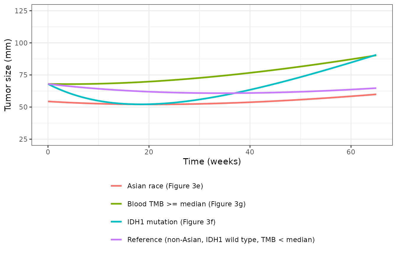
Replicates the categorical panels of Figure 3 (e-g) of Milenkovic-Grisic 2024 for the BTC model, re-anchored at the figure’s 68 mm starting value.
For the BA NSCLC model, the Figure 3i/3j median curve (start about 88
mm, minimum about 55 mm near week 35, about 65 mm at week 65)
corresponds to a typical kg of about 0.88 mm/week rather than the
tabulated 0.728. Under the power form, the cohort medians would then sit
at about (88 / 81.1)^(1 / 0.125) = 1.9 times the CRP
reference and (0.88 / 0.728)^(1 / -0.623) = 0.74 times the
lymphocyte-percentage reference. Those ratios are consistent with the 10
mg/L and 20 percent references chosen here (cohort medians near 19 mg/L
and 15 percent), but the paper does not print the medians, so they are
not used to set the references.
Stochastic simulation
200 virtual patients per model at the reference covariate profile.
rxode2::rxSetSeed(20241304)
nPerArm <- 200L
vgrid <- seq(0, 65, by = 1)
sims <- dplyr::bind_rows(lapply(names(models), function(a) {
  ev <- data.frame(id = rep(seq_len(nPerArm), each = length(vgrid)),
                   time = rep(vgrid, nPerArm)) |>
    dplyr::cross_join(refCov)
  mod <- rxode2::rxode(readModelDb(models[[a]]))
  as.data.frame(rxode2::rxSolve(mod, ev)) |> dplyr::mutate(Arm = a)
}))
#> ℹ parameter labels from comments will be replaced by 'label()'
#> ℹ parameter labels from comments will be replaced by 'label()'
#> ℹ parameter labels from comments will be replaced by 'label()'

vpc <- sims |>
  dplyr::group_by(Arm, time) |>
  dplyr::summarise(
    q05 = stats::quantile(sim, 0.05), q50 = stats::median(sim),
    q95 = stats::quantile(sim, 0.95), .groups = "drop"
  )
ggplot(vpc, aes(time, q50)) +
  geom_ribbon(aes(ymin = q05, ymax = q95), alpha = 0.25, fill = "steelblue") +
  geom_line(linewidth = 1, colour = "steelblue4") +
  facet_wrap(~Arm) +
  labs(x = "Time since first dose (weeks)", y = "Tumor size (mm)") +
  theme_bw()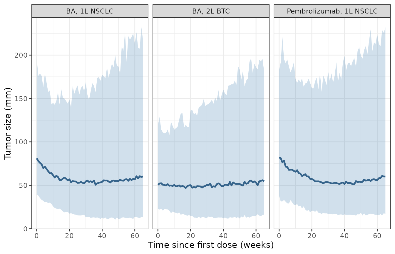
Simulated tumor size (median and 90% prediction interval, with residual error) for 200 patients per model at the reference covariate profile.
Replicating Figure 2 (distribution of ks and kg)
Figure 2 shows box plots of the individual (post hoc) ks and kg in the three analyses. The medians below were read off Figure 2 by the maintainers. The post hoc estimates carry each patient’s own covariates, whereas the simulation holds every patient at the reference profile, so only a broad agreement of the centre is expected.
indiv <- sims |>
  dplyr::filter(time == 0) |>
  dplyr::group_by(Arm) |>
  dplyr::summarise(
    kg_med = stats::median(p), kg_q25 = stats::quantile(p, 0.25), kg_q75 = stats::quantile(p, 0.75),
    ks_med = stats::median(kse), ks_q25 = stats::quantile(kse, 0.25), ks_q75 = stats::quantile(kse, 0.75),
    .groups = "drop"
  ) |>
  dplyr::left_join(
    tibble::tibble(
      Arm = names(models),
      kg_fig2 = c(0.80, 0.85, 0.70),
      ks_fig2 = c(0.016, 0.039, 0.029)
    ),
    by = "Arm"
  )
indiv |>
  dplyr::rename(
    "kg median (sim)" = kg_med, "kg Q1 (sim)" = kg_q25, "kg Q3 (sim)" = kg_q75,
    "kg median (Figure 2)" = kg_fig2,
    "ks median (sim)" = ks_med, "ks Q1 (sim)" = ks_q25, "ks Q3 (sim)" = ks_q75,
    "ks median (Figure 2)" = ks_fig2
  ) |>
knitr::kable(digits = 4)| Arm | kg median (sim) | kg Q1 (sim) | kg Q3 (sim) | ks median (sim) | ks Q1 (sim) | ks Q3 (sim) | kg median (Figure 2) | ks median (Figure 2) |
|---|---|---|---|---|---|---|---|---|
| BA, 1L NSCLC | 0.7871 | 0.3873 | 1.5468 | 0.0361 | 0.0274 | 0.0551 | 0.85 | 0.039 |
| BA, 2L BTC | 0.5990 | 0.3802 | 0.8893 | 0.0174 | 0.0095 | 0.0311 | 0.80 | 0.016 |
| Pembrolizumab, 1L NSCLC | 0.6959 | 0.3891 | 1.1443 | 0.0321 | 0.0202 | 0.0500 | 0.70 | 0.029 |
# Centre-only check: a mis-transcribed typical value or a wrong IIV scale
# moves the simulated median well outside this band.
stopifnot(
  all(abs(log(indiv$kg_med / indiv$kg_fig2)) < log(1.5)),
  all(abs(log(indiv$ks_med / indiv$ks_fig2)) < log(1.5))
)
The paper’s Discussion states that tumor shrinkage was 59% slower in
BTC than in NSCLC. The typical values give
1 - 0.0159 / 0.0368 = 57% against the BA NSCLC model,
consistent with that statement.
PKNCA
Not applicable: the models describe tumor size only. Drug exposure
enters the BTC model as a user-supplied covariate
(AUC_BINTRAFUSP_REL) derived from a separate bintrafusp
alfa population PK model, and no concentration-time profile is
simulated, so there is no non-compartmental analysis to compare
against.
Assumptions and deviations
-
Covariate equation forms are not printed. Neither
the article nor Data S1 states how the covariates enter the model or the
reference values of the continuous covariates. The maintainers encoded:
- the three BTC categorical effects (Asian race on BTS, IDH1 on ks and
kg, blood TMB at or above the median on kg) as fractional changes
P * (1 + theta * indicator), the form that reproduces Figure 3e-g (see above); - every continuous covariate as a power effect
(cov / ref)^theta, with rounded standard reference values because no cohort median is reported: minor allele frequency 1 percent, time since diagnosis 365 days, AST 30 U/L, CRP 10 mg/L, lymphocytes 20 percent of leukocytes. The units of minor allele frequency, time since diagnosis and CRP are also not reported (assumed percent, days and mg/L); - the BA exposure effect as linear in the dynamic AUC normalised to
the analysis-population median,
ks * (1 + 0.339 * (AUC_BINTRAFUSP_REL - 1)). The paper gives neither the AUC units, the time window nor the form; the dimensionless coefficient is only interpretable against a normalised exposure, and the Figure 3 median curve reaches its minimum where the tabulated ks applies.
- the three BTC categorical effects (Asian race on BTS, IDH1 on ks and
kg, blood TMB at or above the median on kg) as fractional changes
- Typical values belong to an unreported reference profile. Figure 3 median curves start at about 68 mm (BTC) and 88 mm (BA NSCLC) rather than at the tabulated 51.3 and 81.1 mm. With the reference values above, a patient at the cohort medians will therefore not, in general, reproduce the Figure 3 median curve; the size of the offset depends on the unreported cohort medians.
-
Minor allele frequency is described as “minor
allele frequency for all detected somatic variants in the sample”;
whether the sample is plasma ctDNA or tumor tissue is not stated. It is
carried in the
CTDNA_VAFcolumn. Values must be greater than 0 for the power form. -
Residual error is reported as a proportional %CV of
a log-transform-both-sides additive error; the log-scale SD is taken as
%CV / 100 (0.156, 0.128 and 0.113) and encoded with
lnorm(). - Exposure in NSCLC. BA and pembrolizumab exposure were tested and not retained in the NSCLC models, so neither NSCLC file carries an exposure input.
- Upstream PK. The BTC model needs an individual dynamic AUC from the BA population PK model of Vugmeyster 2022 (Cancer Chemother Pharmacol 90:369-379), which is not packaged in nlmixr2lib.
- Literature check. No erratum or correction for this article was found in Europe PMC (checked 2026-11-07).