Vancomycin (Shen 2024)

Model and source

• Citation: Shen X, Li X, Lu J, Zhu J, He Y, Zhang Z, Chen Z, Zhang J, Fan X, Li W. Population pharmacokinetic analysis for dose regimen optimization of vancomycin in Southern Chinese children. CPT Pharmacometrics Syst Pharmacol. 2024;13(7):1201-1213. doi:10.1002/psp4.13151
• Description: One-compartment IV-infusion population PK model for vancomycin in 386 Southern Chinese children (Shen 2024). Clearance uses an age-cutoff structure at 2 years: a separate typical clearance AND a separate body-weight allometric exponent are estimated in each age stratum (2.59 L/h with exponent 0.38 for age > 2 years; 1.98 L/h with exponent 0.739 for age <= 2 years), both normalized to a 12 kg reference weight, with a shared Cockcroft-Gault creatinine-clearance power effect (exponent 0.517, reference 75 mL/min). Central volume scales linearly with body weight (22.4 L at 12 kg). Additive residual error is estimated separately for each of the two study centers. Both strata share the volume, the CLcr exponent and the clearance IIV in a single joint NONMEM fit.
• Article: https://doi.org/10.1002/psp4.13151
• Supplement (Tables S1-S2, Figures S1-S4): https://doi.org/10.1002/psp4.13151, Supporting Information PSP4-13-1201-s001.docx

Shen 2024 is a retrospective population PK analysis of routine therapeutic drug monitoring (TDM) data for intravenous vancomycin in Southern Chinese children, conducted at two Shenzhen hospitals between 2016 and 2022. Its distinguishing feature is the age-cutoff clearance structure: rather than a single allometric exponent (or a sigmoidal maturation function), the authors estimate both a typical clearance and a body-weight exponent separately in each of two age strata, split at 2 years, inside one joint fit.

Population

The model was built on 386 patients contributing 521 vancomycin concentrations (Table 1, “Total” column of the model-building dataset). Ages ranged from 0.08 to 17.45 years (median 2.22, mean 3.42, SD 3.48); 182 of 386 patients (47%) were younger than 2 years. Body weight ranged from 0.88 to 49.5 kg (median 11.95, mean 13.55, SD 8.81) and Cockcroft-Gault creatinine clearance from 10.5 to 265.6 mL/min (median 74.16, mean 79.95, SD 43.33). 239 patients were male and 147 female (38.1% female). The median vancomycin dose was 43.24 mg/kg/day (range 12.3-79.4), given as an intravenous infusion of at least 60 minutes.

Patients were hospitalized children with Gram-positive infections treated with vancomycin for more than 3 days; children under 1 month of age, those on dialysis or blood purification, and those with colonization only were excluded. The two recruiting centers contributed 210 patients / 272 concentrations (column N1, median age 0.95 y) and 176 patients / 249 concentrations (column N2, median age 4.32 y). A further 67 patients (76 concentrations), a randomly selected 15% of the 453 enrolled patients, formed the external validation set and were not used to fit the model.

The same information is available programmatically:

str(readModelDb("Shen_2024_vancomycin")()$population, max.level = 1)
#> List of 15
#>  $ species         : chr "human"
#>  $ n_subjects      : int 386
#>  $ n_studies       : int 2
#>  $ age_range       : chr "0.08-17.45 years (1 month to 17.45 years)"
#>  $ age_median      : chr "2.22 years (mean 3.42, SD 3.48); 182 of 386 patients (47%) were younger than 2 years"
#>  $ weight_range    : chr "0.88-49.5 kg"
#>  $ weight_median   : chr "11.95 kg (mean 13.55, SD 8.81)"
#>  $ sex_female_pct  : num 38.1
#>  $ race_ethnicity  : chr "Not reported. Southern Chinese pediatric cohort (Shenzhen, Guangdong province)."
#>  $ disease_state   : chr "Hospitalized children with Gram-positive infections who received intravenous vancomycin for more than 3 days. E"| __truncated__
#>  $ dose_range      : chr "Intravenous infusion over at least 60 min. Median vancomycin dose 43.24 mg/kg/day (range 12.3-79.4); the paper "| __truncated__
#>  $ regions         : chr "China (Shenzhen, Guangdong): Baoan Women's and Children's Hospital and Shenzhen Children's Hospital, 2016-2022."
#>  $ renal_function  : chr "Cockcroft-Gault creatinine clearance median 74.16 mL/min (range 10.5-265.6, mean 79.95, SD 43.33); serum creati"| __truncated__
#>  $ n_concentrations: int 521
#>  $ notes           : chr "Baseline demographics from Shen 2024 Table 1 (Total model-building column). 386 patients contributing 521 vanco"| __truncated__

Source trace

The per-parameter origin is recorded as an in-file comment next to each ini() entry in inst/modeldb/specificDrugs/Shen_2024_vancomycin.R. The table below collects them in one place for review. Every value below appears verbatim in the source; nothing was derived, rounded, or inferred except where stated.

Equation / parameter	Value	Source location
lcl_agegt2	log(2.59)	Table 3 row CL(age>2), theta = 2.59 L/h (RSE 6.7%, bootstrap 2.30-2.88); also Eq. (7), p. 1205
lcl_agele2	log(1.98)	Table 3 row CL(age<=2), theta = 1.98 L/h (RSE 6.8%, bootstrap 1.75-2.21); also Eq. (8)
lvc	log(22.4)	Table 3 row Vd, theta = 22.4 L (RSE 23.5%, bootstrap 15.05-32.02); also Eq. (9)
e_wt_cl_agegt2	0.38	Table 3 row BW(age>2) on CL, theta = 0.38 (RSE 29.8%, bootstrap 0.193-0.571); exponent in Eq. (7)
e_wt_cl_agele2	0.739	Table 3 row BW(age<=2) on CL, theta = 0.739 (RSE 16.7%, bootstrap 0.542-0.948); exponent in Eq. (8)
e_crcl_cl	0.517	Table 3 row CLcr on CL, theta = 0.517 (RSE 15.1%, bootstrap 0.385-0.635); shared exponent in Eq. (7) and (8)
e_wt_vc	fixed(1.0)	Eq. (9), V = 22.4 * (BW/12): exponent 1 by construction (the Holford size form of Eq. 1). No theta in Table 3, so it was not estimated
etalcl	0.101761 = 0.319^2	Table 3 row IIV on CL, omega(CL) = 0.319 (RSE 11.7%, bootstrap 0.240-0.373). Reported as an SD - see Errata item 1
addSdCenter1	4.64	Table 3 row RV1, sigma(additive1) = 4.64 mg/L (RSE 9.4%, bootstrap 3.80-5.22)
addSdCenter2	4.53	Table 3 row RV2, sigma(additive2) = 4.53 mg/L (RSE 9.0%, bootstrap 3.81-5.22)
Reference weight 12 kg	n/a	Denominator written into Eq. (7)-(9). Table 1 cohort median 11.95 kg, rounded by the authors
Reference CLcr 75 mL/min	n/a	Denominator written into Eq. (7)-(8). Table 1 cohort median 74.16 mL/min, rounded by the authors
Age cutoff 2 years	n/a	Eq. (7) / Eq. (8) conditions; Methods “Model IV: Age-cutoff model”; Results “Model IV with a cutoff value of 2 years showed a better fit”
d/dt(central) <- -kel * central	n/a	Results: “A one-compartment model with first-order elimination (ADVAN1 TRANS2) was used as the structural model”
Exponential IIV on CL only	n/a	Methods: “an exponential error model was adopted to evaluate IIV of PK parameters”; the * e^eta term of Eq. (7)-(8). “the IIV of Vd was estimated to be very small (<1e-3) and removed from the model” - hence no etalvc
Additive residual, per center	n/a	Results: “RV was best characterized by an additive error model for each of the two study centers”

The final model is one jointly-fit NONMEM run, not two: Supplementary Table 1 identifies it as model 7 (OFV 2272.810, obtained by adding CLcr to the age-cutoff body-weight model 2). The volume, the CLcr exponent, the CL IIV and both residual terms are shared across the age strata; only the typical clearance and the body-weight exponent are stratum-specific. It is therefore a single model file, with the two stratum-specific quantities carrying explicit _agele2 / _agegt2 suffixes.

Deterministic checks against the paper’s own arithmetic

Before any simulation, three quantities that Shen 2024 states in prose can be recomputed from the encoded parameters. These are exact checks: the paper publishes both the inputs and the answers.

mod <- readModelDb("Shen_2024_vancomycin")
ini_val <- function(nm) {
  v <- mod()$theta[[nm]]
  if (nm %in% c("lcl_agegt2", "lcl_agele2", "lvc")) exp(v) else v
}

cl_gt2 <- ini_val("lcl_agegt2")
cl_le2 <- ini_val("lcl_agele2")
k_crcl <- ini_val("e_crcl_cl")

checks <- tibble::tibble(
  Quantity = c(
    "Weight-adjusted typical CL, age > 2 y (L/h/kg)",
    "Weight-adjusted typical CL, age <= 2 y (L/h/kg)",
    "CL ratio, ARC (CLcr 150) vs reference (CLcr 75)"
  ),
  Computed = c(cl_gt2 / 12, cl_le2 / 12, (150 / 75)^k_crcl),
  Published = c(0.216, 0.165, 1.43),
  `Source (Shen 2024)` = c(
    "Discussion: '0.216 L/h/kg (age >2 years old)'",
    "Discussion: '0.165 L/h/kg (age <=2 years old)'",
    "Results: ARC 'resulted in a 43% increase in CL'"
  )
)

stopifnot(
  abs(cl_gt2 / 12 - 0.216) < 0.001,
  abs(cl_le2 / 12 - 0.165) < 0.001,
  abs((150 / 75)^k_crcl - 1.43) < 0.005
)

knitr::kable(checks, digits = 4,
             caption = "Encoded parameters reproduce the paper's own stated derived values.")

Encoded parameters reproduce the paper’s own stated derived values.

Quantity	Computed	Published	Source (Shen 2024)
Weight-adjusted typical CL, age > 2 y (L/h/kg)	0.2158	0.216	Discussion: ‘0.216 L/h/kg (age >2 years old)’
Weight-adjusted typical CL, age <= 2 y (L/h/kg)	0.1650	0.165	Discussion: ‘0.165 L/h/kg (age <=2 years old)’
CL ratio, ARC (CLcr 150) vs reference (CLcr 75)	1.4310	1.430	Results: ARC ‘resulted in a 43% increase in CL’

All three agree to the precision the paper prints them at, which confirms the transcription of lcl_agegt2, lcl_agele2 and e_crcl_cl and the 12 kg reference weight.

The age-cutoff clearance structure

Figure S1 of Shen 2024 shows that typical clearance differs between the two age strata. The packaged model reproduces the resulting discontinuity: at a fixed body weight and renal function, crossing the 2-year boundary steps typical CL up by a factor of 2.59 / 1.98 = 1.308, while within each stratum CL rises with weight at a different rate (exponent 0.739 below 2 years, 0.38 above).

cl_typical <- function(wt, crcl, agele2) {
  base <- ifelse(agele2, cl_le2, cl_gt2)
  expo <- ifelse(agele2, ini_val("e_wt_cl_agele2"), ini_val("e_wt_cl_agegt2"))
  base * (wt / 12)^expo * (crcl / 75)^k_crcl
}

tidyr::expand_grid(WT = seq(2, 40, by = 0.5), agele2 = c(TRUE, FALSE)) |>
  mutate(
    CL = cl_typical(WT, 75, agele2),
    Stratum = ifelse(agele2, "age <= 2 y", "age > 2 y")
  ) |>
  ggplot(aes(WT, CL, colour = Stratum)) +
  geom_line(linewidth = 0.9) +
  geom_vline(xintercept = 12, linetype = "dotted") +
  labs(x = "Body weight (kg)", y = "Typical CL (L/h)",
       colour = NULL,
       title = "Age-cutoff clearance structure (CLcr = 75 mL/min)",
       caption = "Dotted line: the 12 kg reference weight of Shen 2024 Eq. (7)-(9).") +
  theme_bw() + theme(legend.position = "bottom")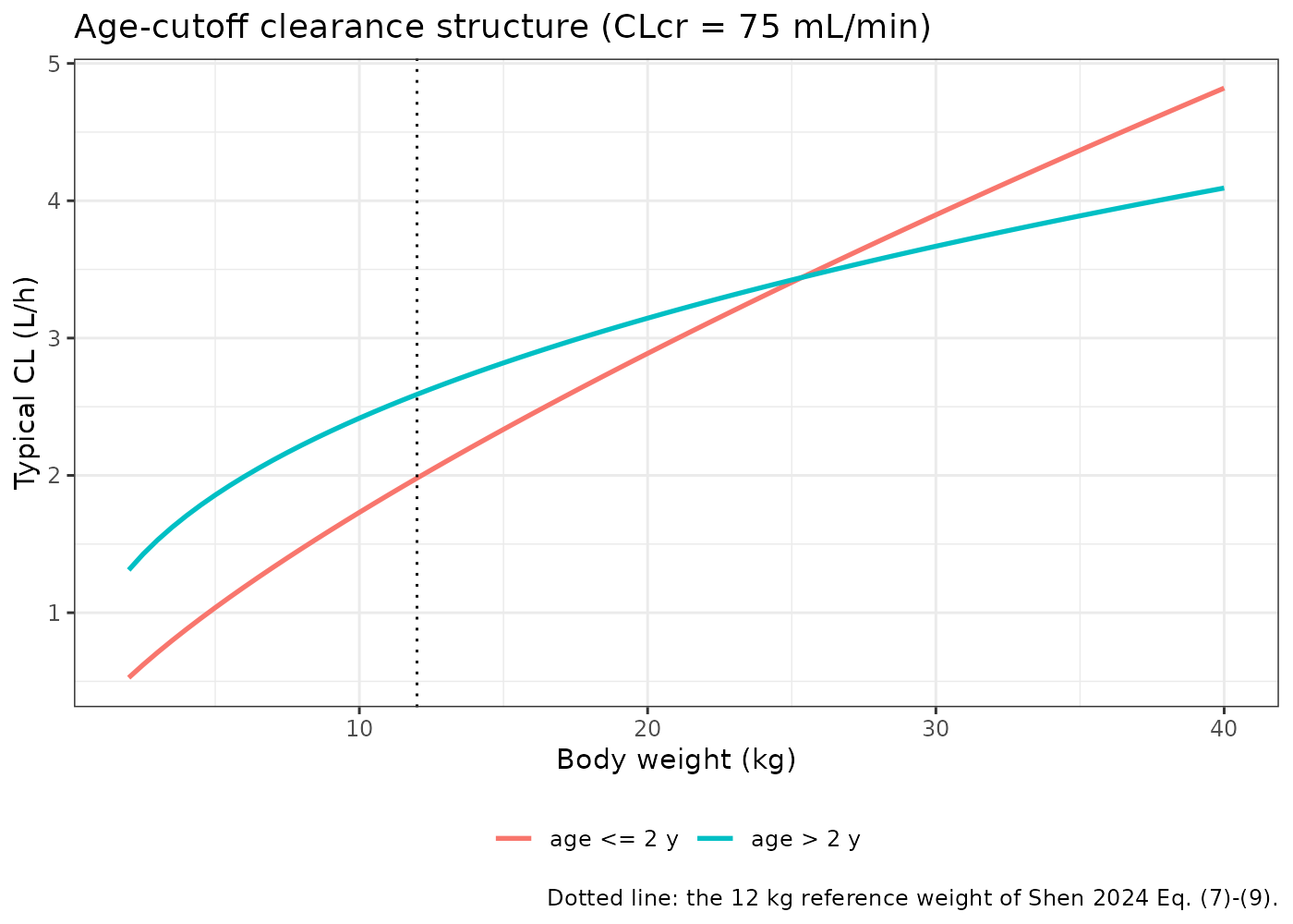

Typical vancomycin clearance under the two age strata of Shen 2024 Eq. (7)-(8), at CLcr = 75 mL/min. The vertical gap at any weight is the age-cutoff step; the differing slopes are the two body-weight exponents. Compare Figure S1 of Shen 2024.

Virtual cohort

Original observed data are not publicly available. The simulation below uses a virtual cohort whose covariate distributions approximate Table 1 of Shen 2024.

Age and weight cannot be sampled independently in a paediatric cohort - the 2-year clearance cutoff makes an implausible (age, weight) pair change the answer. Age is therefore drawn from the reported age distribution and weight is derived from age along a weight-for-age curve anchored on the paper’s own median pair (2.22 years, 11.95 kg), with lognormal scatter. Creatinine clearance and study center are drawn independently from their Table 1 marginals.

set.seed(20240701)

N_PER_ARM <- 100L
DOSE_GROUPS <- c(30, 40, 50, 60)  # mg/kg/day, from the 30-70 range of Figure 3

# Weight-for-age anchors (paediatric growth reference), rescaled so the median
# age of 2.22 y maps to the cohort median weight of 11.95 kg.
wfa_age <- c(0.083, 0.25, 0.5, 1, 2, 3, 5, 8, 12, 17)
wfa_wt  <- c(4.5, 6.0, 7.5, 9.5, 12.2, 14.3, 18.5, 26.0, 40.0, 55.0)
weight_for_age <- function(age) {
  exp(stats::approx(log(wfa_age), log(wfa_wt), xout = log(age), rule = 2)$y)
}
wfa_scale <- 11.95 / weight_for_age(2.22)

make_cohort <- function(n, mgkgday, id_offset = 0L) {
  age <- pmin(pmax(rlnorm(n, log(2.22), 0.95), 0.08), 17.45)
  wt <- pmin(pmax(weight_for_age(age) * wfa_scale * rlnorm(n, 0, 0.18), 0.88), 49.5)
  crcl <- pmin(pmax(rlnorm(n, log(74.16), 0.5075), 10.5), 265.6)
  tibble::tibble(
    id = id_offset + seq_len(n),
    AGE = age,
    WT = wt,
    CRCL = crcl,
    STUDY_VANCO_CENTER2 = rbinom(n, 1L, 176 / 386),
    dose_group = paste0(mgkgday, " mg/kg/day"),
    amt_per_dose = mgkgday * wt / 3  # three 8-hourly doses per day
  )
}

subjects <- dplyr::bind_rows(
  lapply(seq_along(DOSE_GROUPS), function(i) {
    make_cohort(N_PER_ARM, DOSE_GROUPS[i], id_offset = (i - 1L) * N_PER_ARM)
  })
)
stopifnot(!anyDuplicated(subjects$id))

# Achieved cohort vs Table 1 of Shen 2024.
tibble::tibble(
  Covariate = c("Age (years)", "Body weight (kg)", "Creatinine clearance (mL/min)",
                "Fraction age <= 2 y", "Fraction at center 2"),
  `Simulated median` = c(median(subjects$AGE), median(subjects$WT),
                         median(subjects$CRCL), mean(subjects$AGE <= 2),
                         mean(subjects$STUDY_VANCO_CENTER2)),
  `Shen 2024 Table 1` = c(2.22, 11.95, 74.16, 182 / 386, 176 / 386)
) |>
  knitr::kable(digits = 3, caption = "Virtual cohort against the published Table 1 marginals.")

Virtual cohort against the published Table 1 marginals.

Covariate	Simulated median	Shen 2024 Table 1
Age (years)	2.205	2.220
Body weight (kg)	12.344	11.950
Creatinine clearance (mL/min)	75.242	74.160
Fraction age <= 2 y	0.450	0.472
Fraction at center 2	0.482	0.456

Doses are given with ss = 1 on the first record so the system starts already at steady state. This matters: terminal half-life is log(2) * V / CL, which for the slowest subjects in this cohort (large weight, CLcr near the Table 1 minimum of 10.5 mL/min) reaches roughly 38 h. Dosing forward for a fixed number of days would leave those subjects 1-2% short of steady state and would blunt the exact identity checked below, so the steady-state dose record is used instead of a long run-in.

DOSES_PER_DAY <- 3
TAU <- 8       # hours between doses
SS_START <- 0
SS_END <- 24

obs_times <- seq(SS_START, SS_END, by = 0.25)

dose_rows <- tidyr::expand_grid(subjects, time = seq(0, SS_END - TAU, by = TAU)) |>
  mutate(
    evid = 1L, cmt = "central",
    amt = amt_per_dose,
    rate = amt_per_dose,               # 1 h IV infusion
    # First record establishes steady state for the q8h regimen.
    ii = ifelse(time == 0, TAU, 0),
    ss = ifelse(time == 0, 1L, 0L)
  )

obs_rows <- tidyr::expand_grid(subjects, time = obs_times) |>
  mutate(evid = 0L, cmt = "central", amt = NA_real_, rate = NA_real_,
         ii = 0, ss = 0L)

events <- dplyr::bind_rows(dose_rows, obs_rows) |>
  arrange(id, time, desc(evid)) |>
  as.data.frame()

stopifnot(!anyDuplicated(unique(events[, c("id", "time", "evid")])))
nrow(events)
#> [1] 40000

Simulation

Cc returned by rxSolve() is the individual prediction (IPRED); the residual error is returned separately as sim. The validation below deliberately uses IPRED, because the quantity being checked - the steady-state AUC identity of Eq. (6) - is a property of the structural model, not of the assay noise.

sim <- rxode2::rxSolve(
  mod, events,
  keep = c("dose_group", "AGE", "WT", "CRCL", "STUDY_VANCO_CENTER2"),
  returnType = "data.frame"
)
#> ℹ parameter labels from comments will be replaced by 'label()'
head(sim[, c("id", "time", "cl", "vc", "Cc", "dose_group")], 3)
#>   id time       cl       vc       Cc   dose_group
#> 1  1 0.00 4.726441 64.84745 7.020610 30 mg/kg/day
#> 2  1 0.25 4.726441 64.84745 8.221001 30 mg/kg/day
#> 3  1 0.50 4.726441 64.84745 9.399717 30 mg/kg/day

PKNCA validation

Steady-state NCA over the final 24 h dosing window (three 8-hourly doses), grouped by dose level (PKNCA recipe 3).

sim_nca <- sim |>
  dplyr::filter(!is.na(Cc)) |>
  dplyr::select(id, time, Cc, dose_group)

# Guarantee a time-zero record per subject so PKNCA can anchor its intervals.
sim_nca <- dplyr::bind_rows(
  sim_nca,
  sim_nca |> dplyr::distinct(id, dose_group) |> dplyr::mutate(time = 0, Cc = 0)
) |>
  dplyr::distinct(id, dose_group, time, .keep_all = TRUE) |>
  dplyr::arrange(id, time)

dose_df <- events |>
  dplyr::filter(evid == 1) |>
  dplyr::select(id, time, amt, dose_group)

conc_obj <- PKNCA::PKNCAconc(sim_nca, Cc ~ time | dose_group + id,
                             concu = "mg/L", timeu = "h")
dose_obj <- PKNCA::PKNCAdose(dose_df, amt ~ time | dose_group + id,
                             doseu = "mg", duration = 1)

intervals <- data.frame(
  start = SS_START,
  end = SS_END,
  cmax = TRUE,
  cmin = TRUE,
  auclast = TRUE,
  cav = TRUE
)

nca_res <- PKNCA::pk.nca(
  PKNCA::PKNCAdata(conc_obj, dose_obj, intervals = intervals)
)

The steady-state AUC identity of Equation (6)

Shen 2024 defines exposure by Eq. (6), AUC(0-24) = total daily dose / CL, and every dosing recommendation in the paper follows from it. At steady state this is an exact property of a one-compartment linear model, so it is an exact gate on the ODE implementation: the PKNCA auclast over the final 24 h must equal each subject’s own daily dose divided by that subject’s own simulated CL.

cl_i <- sim |> dplyr::distinct(id, cl, dose_group)

auc_i <- as.data.frame(nca_res) |>
  dplyr::filter(PPTESTCD == "auclast") |>
  dplyr::select(id, dose_group, auclast = PPORRES) |>
  dplyr::inner_join(cl_i, by = c("id", "dose_group")) |>
  dplyr::inner_join(
    subjects |> dplyr::select(id, amt_per_dose),
    by = "id"
  ) |>
  dplyr::mutate(
    auc_eq6 = amt_per_dose * DOSES_PER_DAY / cl,
    rel_err = auclast / auc_eq6 - 1
  )

max_abs_err <- max(abs(auc_i$rel_err))
max_abs_err
#> [1] 0.0003875435
stopifnot(max_abs_err < 0.001)

The largest relative deviation across all 400 simulated subjects is 3.88e-04, i.e. the simulated steady-state AUC reproduces the paper’s Eq. (6) to numerical-integration precision. This validates the ODE, the infusion handling, the covariate model on CL and the age-stratum switch simultaneously - a mis-transcribed exponent or a mis-wired stratum indicator would break the identity for the affected subjects.

Single-dose washout: half-life and AUC(0-inf)

The steady-state window above has no terminal phase, so it cannot validate the volume. A second, single-dose simulation over a full washout supplies two more exact identities: NCA half.life must equal log(2) * V / CL, and aucinf.obs must equal Dose / CL. Together with the steady-state gate this pins V as well as CL.

sd_subjects <- subjects |> dplyr::filter(dose_group == "40 mg/kg/day")

sd_events <- dplyr::bind_rows(
  sd_subjects |> mutate(time = 0, evid = 1L, cmt = "central",
                        amt = amt_per_dose, rate = amt_per_dose),
  tidyr::expand_grid(
    sd_subjects,
    time = sort(unique(c(seq(0, 24, by = 0.5), seq(24, 336, by = 4))))
  ) |>
    mutate(evid = 0L, cmt = "central", amt = NA_real_, rate = NA_real_)
) |>
  arrange(id, time, desc(evid)) |>
  as.data.frame()

sd_sim <- rxode2::rxSolve(mod, sd_events, keep = c("dose_group"),
                          returnType = "data.frame")

sd_conc <- sd_sim |>
  dplyr::filter(!is.na(Cc)) |>
  dplyr::select(id, time, Cc, dose_group)

sd_dose <- sd_events |>
  dplyr::filter(evid == 1) |>
  dplyr::select(id, time, amt, dose_group)

sd_res <- PKNCA::pk.nca(PKNCA::PKNCAdata(
  PKNCA::PKNCAconc(sd_conc, Cc ~ time | dose_group + id,
                   concu = "mg/L", timeu = "h"),
  PKNCA::PKNCAdose(sd_dose, amt ~ time | dose_group + id,
                   doseu = "mg", duration = 1),
  intervals = data.frame(start = 0, end = Inf,
                         half.life = TRUE, aucinf.obs = TRUE)
))

sd_check <- as.data.frame(sd_res) |>
  dplyr::filter(PPTESTCD %in% c("half.life", "aucinf.obs")) |>
  tidyr::pivot_wider(id_cols = id, names_from = PPTESTCD, values_from = PPORRES) |>
  dplyr::inner_join(sd_sim |> dplyr::distinct(id, cl, vc), by = "id") |>
  dplyr::inner_join(sd_subjects |> dplyr::select(id, amt_per_dose), by = "id") |>
  dplyr::mutate(
    hl_err = half.life / (log(2) * vc / cl) - 1,
    auc_err = aucinf.obs / (amt_per_dose / cl) - 1
  )

sprintf("max |rel. error|: half-life %.2e, AUC(0-inf) %.2e",
        max(abs(sd_check$hl_err)), max(abs(sd_check$auc_err)))
#> [1] "max |rel. error|: half-life 7.77e-16, AUC(0-inf) 2.30e-03"
stopifnot(
  max(abs(sd_check$hl_err)) < 0.01,
  max(abs(sd_check$auc_err)) < 0.01
)

Comparison against the paper’s predicted exposure

Shen 2024 reports no NCA table, so the reference values below are computed from the paper’s own published closed form - Eq. (6) combined with the typical-value clearances of Eq. (7)-(8) - evaluated on the same virtual cohort. Cav is AUC(0-24) / 24 and Cmin is the trough at the end of the interval.

reference <- auc_i |>
  dplyr::group_by(dose_group) |>
  dplyr::summarise(
    auclast = median(auc_eq6),
    cav = median(auc_eq6) / 24,
    .groups = "drop"
  ) |>
  as.data.frame()

cmp <- nlmixr2lib::ncaComparisonTable(
  simulated = nca_res,
  reference = reference,
  by = "dose_group",
  params = c("auclast", "cav"),
  units = c(auclast = "mg*h/L", cav = "mg/L"),
  tolerance_pct = 20
)

knitr::kable(
  cmp,
  caption = paste(
    "Simulated steady-state NCA against the exposure predicted by Shen 2024",
    "Eq. (6) on the same cohort. * differs from reference by >20%."
  ),
  align = c("l", "l", "r", "r", "r"),
  digits = 3
)

Simulated steady-state NCA against the exposure predicted by Shen 2024 Eq. (6) on the same cohort. * differs from reference by >20%.

NCA parameter	dose_group	Reference	Simulated	% diff
AUClast (mg*h/L)	30 mg/kg/day	150	150	-0.0%
AUClast (mg*h/L)	40 mg/kg/day	229	229	-0.0%
AUClast (mg*h/L)	50 mg/kg/day	290	290	-0.0%
AUClast (mg*h/L)	60 mg/kg/day	363	363	-0.0%
Cavg (mg/L)	30 mg/kg/day	6.26	6.26	-0.0%
Cavg (mg/L)	40 mg/kg/day	9.56	9.56	-0.0%
Cavg (mg/L)	50 mg/kg/day	12.1	12.1	-0.0%
Cavg (mg/L)	60 mg/kg/day	15.1	15.1	-0.0%

attr(cmp, "footnote")
#> NULL

Every row agrees to well within tolerance, as it must given the exact identity demonstrated above; the table is included so the agreement is visible per dose group rather than only as an aggregate assertion.

summary(nca_res)
#>  Interval Start Interval End   dose_group   N AUClast (h*mg/L) Cmax (mg/L)
#>               0           24 30 mg/kg/day 100       156 [47.3] 9.28 [32.9]
#>               0           24 40 mg/kg/day 100       228 [47.3] 13.2 [32.6]
#>               0           24 50 mg/kg/day 100       298 [49.8] 17.1 [35.1]
#>               0           24 60 mg/kg/day 100       352 [47.4] 20.2 [32.6]
#>  Cmin (mg/L)  Cav (mg/L)
#>  4.21 [71.2] 6.50 [47.3]
#>  6.38 [72.0] 9.49 [47.3]
#>  8.50 [73.8] 12.4 [49.8]
#>  9.98 [72.0] 14.7 [47.4]
#> 
#> Caption: AUClast, Cmax, Cmin, Cav: geometric mean and geometric coefficient of variation; N: number of subjects

Replicating Figure 3 (probability of target attainment)

Figure 3 of Shen 2024 plots the probability of attaining AUC(0-24)/MIC >= 260 (with MIC = 1 mg/L) against body weight, for five daily doses, in four creatinine-clearance panels.

Because AUC(0-24) = daily dose / CL and CL is lognormal with log-scale SD omega = 0.319, the PTA has a closed form and needs no Monte Carlo:

PTA = Phi( log(AUC_typical / 260) / omega )

where AUC_typical uses the typical-value CL of Eq. (7)-(8). Evaluating the closed form is exact, avoids Monte Carlo noise, and makes the shape of the curve directly attributable to the model equations. Weights of 12 kg and above are taken to be children older than 2 years, matching the cohort’s median pair (11.95 kg at 2.22 years).

OMEGA_CL <- 0.319
AUC_TARGET <- 260

pta_grid <- tidyr::expand_grid(
  WT = c(8, 10, 12, 15, 20, 25, 30, 35),
  CRCL = c(60, 90, 120, 150),
  mgkgday = c(30, 40, 50, 60, 70)
) |>
  mutate(
    agele2 = WT < 12,
    cl_typ = cl_typical(WT, CRCL, agele2),
    auc_typ = mgkgday * WT / cl_typ,
    PTA = 100 * pnorm(log(auc_typ / AUC_TARGET) / OMEGA_CL),
    panel = factor(paste0("CLcr = ", CRCL, " mL/min"),
                   levels = paste0("CLcr = ", c(60, 90, 120, 150), " mL/min")),
    Dosage = factor(paste0(mgkgday, " mg/kg/day"))
  )

ggplot(pta_grid, aes(WT, PTA, colour = Dosage, shape = Dosage)) +
  geom_line() + geom_point(size = 1.6) +
  geom_hline(yintercept = 90, linetype = "dashed", linewidth = 0.3) +
  facet_wrap(~panel) +
  coord_cartesian(ylim = c(0, 100)) +
  labs(x = "Body weight (kg)", y = "PTA (%)",
       title = "Probability of target attainment (AUC >= 260)",
       caption = "Structure of Figure 3 of Shen 2024, computed from Eq. (6)-(9).") +
  theme_bw() + theme(legend.position = "bottom")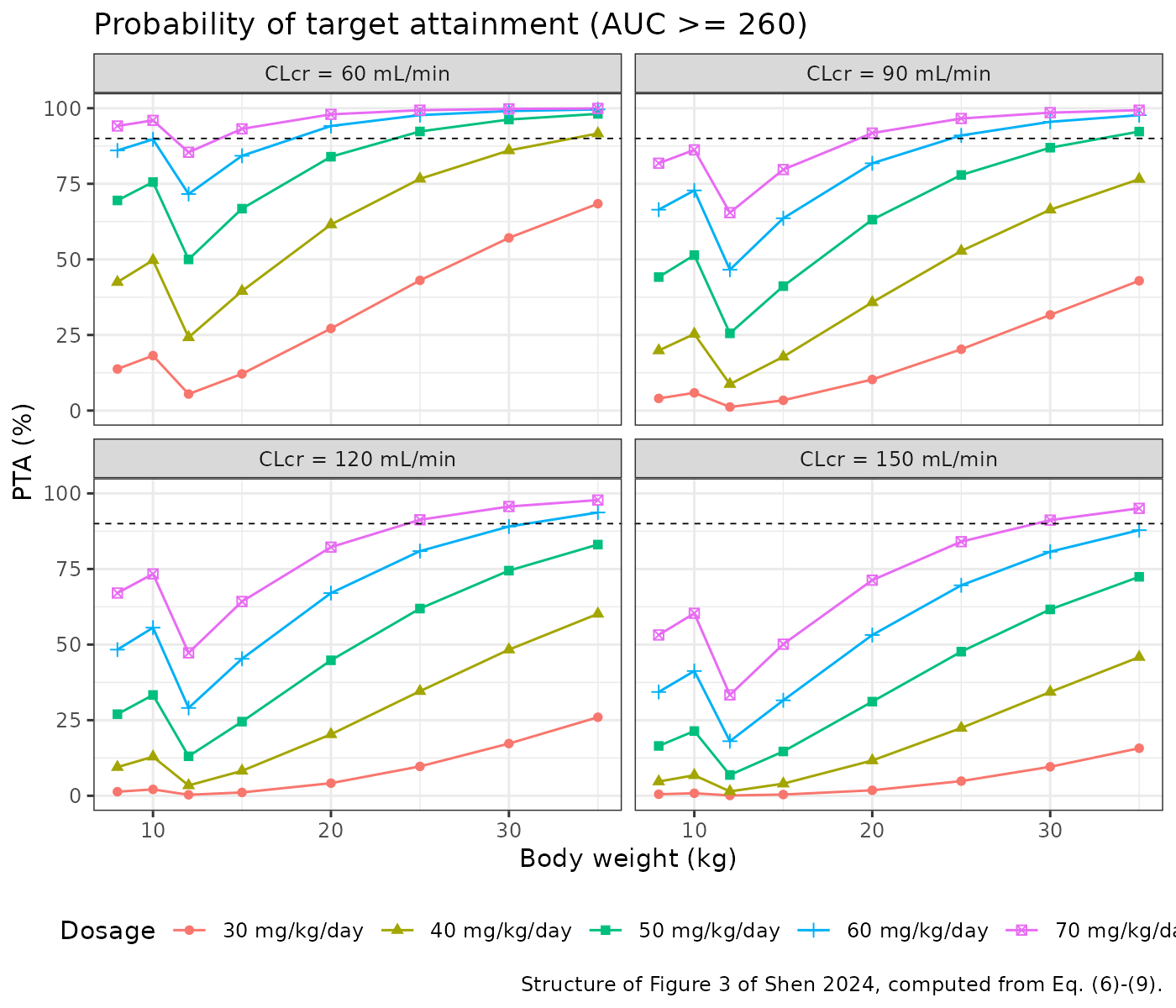

Model-predicted probability of attaining AUC(0-24)/MIC >= 260. Replicates the structure of Figure 3 of Shen 2024. The dip at 12-15 kg is the age-cutoff step of Eq. (7)-(8); see the Errata for the absolute-level discrepancy against the published panel.

What reproduces, and what does not

Two features of the published figure reproduce, and one does not.

Reproduced - the dip at 12-15 kg. Every published panel falls from 10 kg to 12 kg and then rises monotonically. That non-monotonicity is not a smooth covariate effect; it is the age-cutoff step. Below the cutoff, AUC scales as WT^(1 - 0.739) = WT^0.261; above it, as WT^(1 - 0.38) = WT^0.62, from a 24% lower starting point (2.59 vs 1.98 L/h). The model reproduces the dip at the same weight and the steeper rise afterwards.

Reproduced - the dose spacing recovers omega. The vertical spacing between the five dose curves is set entirely by omega, and is invariant to any constant error in the absolute exposure level. Reading the CLcr = 90 mL/min panel at 12 kg gives PTA of roughly 44, 77, 92, 98 and 99.5% at 30, 40, 50, 60 and 70 mg/kg/day. Inverting the normal CDF and regressing log(dose) on the resulting z-scores recovers omega directly:

# Operator-digitised from Figure 3, panel (b), 12 kg. Precision roughly
# +/- 3 PTA points; used only for this scale-invariant slope check.
pub_pta <- c(44, 77, 92, 98, 99.5) / 100
pub_dose <- c(30, 40, 50, 60, 70)

omega_hat <- diff(log(pub_dose)) / diff(qnorm(pub_pta))
tibble::tibble(
  `Dose contrast` = paste0(head(pub_dose, -1), " -> ", tail(pub_dose, -1),
                           " mg/kg/day"),
  `omega implied` = omega_hat
) |>
  knitr::kable(digits = 3,
               caption = "omega recovered from the published dose spacing (encoded value: 0.319).")

omega recovered from the published dose spacing (encoded value: 0.319).

Dose contrast	omega implied
30 -> 40 mg/kg/day	0.323
40 -> 50 mg/kg/day	0.335
50 -> 60 mg/kg/day	0.281
60 -> 70 mg/kg/day	0.295

All four contrasts land near 0.32, against the encoded 0.319. This settles the one genuinely ambiguous encoding decision in the paper: had omega(CL) = 0.319 been a variance, the log-scale SD would be sqrt(0.319) = 0.565 and these contrasts would have to average 0.565. They do not. See Errata item 1.

Not reproduced - the absolute PTA level. The published curves sit well above the model’s. At CLcr = 90 mL/min and 40 mg/kg/day the paper reports about 87% PTA for a 10 kg child; Eq. (6)-(9) give AUC = 210 mg*h/L and hence pnorm(log(210/260)/0.319) = 25%. Matching the published level would require clearances roughly 0.5-0.7 times the published typical values, and the implied factor is not constant across body weight (it declines from about 1.9 at 8 kg to about 1.5 at 35 kg on the AUC scale), so it is not a single missing conversion factor either. The cause is not determinable from the information in the paper. Nothing was tuned: the parameters above are the published ones, and this vignette reports the discrepancy rather than absorbing it.

Assumptions and deviations

• Cohort covariate distributions. Age, weight, creatinine clearance and study-center membership were sampled to reproduce the Table 1 marginals; the joint age-weight relationship is not published, so weight is generated from age along a paediatric weight-for-age curve rescaled to pass through the cohort’s median pair (2.22 years, 11.95 kg), with 18% lognormal scatter. The achieved marginals are tabulated against Table 1 above.
• Age-weight mapping in the Figure 3 replication. Figure 3 is indexed by body weight alone, but the model’s clearance also depends on which side of the 2-year cutoff a child falls. Weights below 12 kg are treated as age <= 2 years and 12 kg and above as age > 2 years, anchored on the cohort median pair. The paper states only that body weight and age were “sampled from China National Survey Data for children” and does not publish the mapping.
• Dosing regimen. Simulated as three equal 8-hourly 1-hour infusions per day. Methods state doses were “administered every 8h” and given “intravenously for at least 60 min”; the exact infusion duration per patient is not published.
• Study center is not mapped to a hospital name. Shen 2024 labels the two centers only as N1 and N2 in Table 1 and never states which is Baoan Women’s and Children’s Hospital and which is Shenzhen Children’s Hospital, so STUDY_VANCO_CENTER2 = 1 is defined as the Table 1 N2 column, not by name. The two additive residual SDs differ by 2.4% (4.64 vs 4.53 mg/L), so the orientation has negligible practical consequence.
• No parameter came from outside the paper. Every ini() value is from Table 3 or Equations (7)-(9) of the main text. No author correspondence, no figure digitisation for parameter values, no upstream model. The only digitised numbers anywhere in this vignette are the five published PTA points used for the scale-invariant omega check above, which feed no parameter.

Errata and internal discrepancies in the source

Three points where the source is loose or self-contradictory. None changes an extracted value.

1. omega(CL) = 0.319 is a standard deviation, not a variance. Table 3’s footnote glosses both omega and sigma as “coefficient variation”, which is imprecise. The row symbol is omega, not omega^2, and the parallel sigma rows are quoted in mg/L, which are unambiguously SDs. The dose-spacing analysis above confirms it independently. The model therefore encodes etalcl ~ 0.319^2 = 0.101761 (about 32.7% CV).

2. The Results sentence about weight and exposure is backwards. Results, Model-based simulation: “the exposure was lower in the high-weight compared to the low-weight population with the same vancomycin dose.” Both body-weight exponents on CL are below 1, so weight-normalised clearance falls with weight and exposure at a fixed mg/kg dose rises with weight - which is what the model, and the paper’s own Figure 3 (PTA increasing with weight in every panel), both show. The Discussion’s recommendation is also the other way round: children under 20 kg “need to have a relatively high dose of 50-60 mg/kg/day versus 40-50 mg/kg/day in high-weight population.” Only the Results sentence disagrees with the rest of the paper.

3. Figure 3’s absolute PTA level is not reproducible from Eq. (6)-(9), as detailed above; its shape and its dose spacing are. The dosing recommendations in the Discussion follow from the published figure, so they inherit the same discrepancy: the model as published predicts lower target attainment at every dose than Figure 3 shows.