Meropenem in critically ill patients (Yang 2024)

Model and source

• Citation: Yang Y, Wang Y, Zeng W, Zhou J, Xu M, Lan Y, Liu L, Shen J, Zhang C, He Q. Physiologically-based pharmacokinetic/pharmacodynamic modeling of meropenem in critically ill patients. Sci Rep. 2024;14:19249. doi:10.1038/s41598-024-64223-0. PMCID PMC11335869. The reduced disposition parameters encoded here (Vd 23.21 L, CL 12.07 L/h, f 0.98 in Asians with severe infection) are stated in the Results section ‘Monte carlo simulations’; Vd 23.21 L also appears in Table 1 as the parameter-identification result. The PK/PD target 40%fT>MIC, the MIC panel (1, 2, 4, 8, 16 mg/L) and the dosing regimens (1 g q12h and 1 g q8h at 0.5, 4 and 6 h infusion) are Methods ‘Monte carlo simulations’; the resulting PTA curves are Figure 8B (Asians) and Figure S1 (100%fT>MIC, Asians). Supplement Table S2 gives the critically-ill physiological scaling factors applied inside PK-Sim; Table S1 lists the 40 literature PK studies used to build and verify the PBPK model; Table S5 lists the 31 prospective ICU patients.
• Description: PBPK-derived reduced one-compartment model for meropenem in critically ill (severe pneumonia with or without sepsis) adult Asian ICU patients. The source paper built an 18-tissue whole-body PBPK model in PK-Sim v11.2 for healthy adults and extrapolated it to critically ill patients by scaling albumin, alpha-1-acid glycoprotein, hematocrit and GFR; that whole-body structure is a PK-Sim platform model whose ODEs, organ volumes, blood flows and partition coefficients are NOT written out in the publication and are therefore not reproduced here. What IS fully reported, and is what this file encodes, is the reduced disposition model the authors carried out of the PBPK and into their Monte Carlo target-attainment analysis: Vd 23.21 L, CL 12.07 L/h and unbound fraction 0.98 for Asian patients with severe infection (Results, Monte Carlo simulations). Intravenous infusion dosing; linear elimination; no covariates. The PK/PD index is the fraction of the dosing interval during which the free concentration exceeds the MIC (f%T>MIC), with 40%fT>MIC as the primary target and 100%fT>MIC as a stricter alternative; f%T>MIC is computed from the simulated profile rather than integrated as a model state, following the Minichmayr_2024_ceftaroline precedent. Interindividual variability was assumed lognormal on Vd and CL in the Monte Carlo but its magnitude is not reported anywhere in the paper or its supplement, so both etas are encoded as fixed(0); no residual error model was reported.
• Article: https://doi.org/10.1038/s41598-024-64223-0
• Supplement: https://doi.org/10.1038/s41598-024-64223-0 (Supplementary Information, Tables S1-S5 and Figure S1)

What this file does and does not reproduce

Yang 2024 is a two-layer paper, and only one layer is reproducible from the publication. Being explicit about the boundary is the point of this section.

Not reproduced – the whole-body PBPK layer. The authors built an 18 tissue/organ PBPK model in PK-Sim v11.2 for a typical 30-year-old European male, verified it against 12 healthy-adult literature PK studies, then extrapolated it to critically ill patients by scaling four physiological parameters relative to PK-Sim’s healthy control values (Supplementary Table S2): albumin 0.54, alpha-1-acid glycoprotein 1.62, hematocrit 0.77 and GFR 0.50. That structure is a PK-Sim platform model. The paper prints neither the ODE system, nor organ volumes, nor blood flows, nor partition coefficients, and Table S2’s footnote states that the control values the scaling factors multiply are “described in PK-Sim for healthy individuals” – i.e. they are platform internals, not published numbers. Reconstructing that layer would require substituting parameters that appear in no source on disk, which the nlmixr2lib PBPK sourcing rule forbids.

Reproduced – the reduced disposition model. What the authors did publish in full is the reduced model they carried out of the PBPK and into their Monte Carlo target-attainment analysis: Vd 23.21 L, CL 12.07 L/h and unbound fraction 0.98 for Asian patients with severe infection. That is a complete one-compartment intravenous model, and it is the object this vignette validates. It is also the model behind every dosing recommendation the paper actually makes, since those recommendations come from the Monte Carlo PTA analysis rather than from the whole-body simulations directly.

Two independent checks below establish that the reduced parameters really are the paper’s Monte Carlo model rather than an incidental summary: an exact match to a published clearance in different units, and a reproduction of every qualitative conclusion the paper drew from its PTA figure.

Population

The paper draws on three distinct populations, which should not be conflated. The PBPK model was developed for a typical 30-year-old European male using PK-Sim’s virtual population and optimised against five single-dose 1 g studies, then verified against 12 healthy-adult literature PK studies. It was then extrapolated to critically ill patients and verified against 10 literature studies in severe infection. Supplementary Table S1 lists all 40 literature study arms with ethnicity, disease, age, N, sex ratio and regimen.

Separately, a prospective TDM cohort of 92 plasma samples from 31 ICU patients at the Third People’s Hospital of Chengdu provided an external check (Supplementary Table S5): mean age 66 years (range 38-95), mean weight 57 kg (range 42-85 kg among the patients whose weight was recorded), mean serum creatinine 87.06 umol/L, 14 of 31 female. Patients had severe pneumonia with or without sepsis; cirrhosis, any liver damage and renal failure were exclusions, though 6 patients (19.35%) received CRRT during treatment. 71 of the 92 samples (77.17%) fell inside the predicted 5th-95th percentile band (Figure 7).

Finally, the Monte Carlo target-attainment analysis simulated 10,000 virtual patients with Pseudomonas aeruginosa infection using the reduced parameters encoded here.

The same information is available programmatically via readModelDb("Yang_2024_meropenem_pbpk")()$population.

Source trace

The per-parameter origin is recorded as an in-file comment next to each ini() entry in inst/modeldb/specificDrugs/Yang_2024_meropenem_pbpk.R. The table below collects them in one place for review.

Equation / parameter	Value	Source location
lcl (CL)	12.07 L/h	Results, “Monte carlo simulations”: “The Vd, CL, and f were defined as 23.21 L, 12.07 L/h, and 0.98 in Asians with severe infection from PBPK model”
lvc (Vd)	23.21 L	Results, “Monte carlo simulations” (as above); also Table 1, Vd(L) row, source/method “Parameter identification”
fu	0.98	Table 1, ADME block, fu p row (source Martins 2020); re-stated as f in Results, “Monte carlo simulations”
etalcl, etalvc	fixed(0)	Methods, “Monte carlo simulations” declares lognormal (“log-gaussian”) IIV on Vd and CL; the magnitude is not reported anywhere in the paper or supplement
propSd	fixed(0)	No residual error model reported – the PBPK is a forward simulation evaluated by MFE / GMFE, not a likelihood fit
d/dt(central) <- -kel * central	n/a	One-compartment intravenous disposition implied by the Monte Carlo parameterisation (a single Vd and a single CL); infusion durations 0.5, 4 and 6 h per Methods, “Monte carlo simulations”
Cc <- central / vc	n/a	Total plasma concentration
Cfree <- fu * Cc	n/a	Methods, “Monte carlo simulations”: the PK/PD index is f%T > MIC, the time the free fraction exceeds the MIC
PK/PD target	40%fT>MIC	Methods, “Monte carlo simulations”: “40%fT > MIC was used as the target threshold”; 100%fT>MIC alternative in Discussion and Figure S1
MIC panel	1, 2, 4, 8, 16 mg/L	Methods, “Monte carlo simulations”
Regimens	1 g q12h, 1 g q8h; 0.5, 4, 6 h infusion	Methods, “Monte carlo simulations”

Virtual cohort

This model carries no covariates, and its two IIV terms are fixed(0) because the paper never published their magnitudes (see Errata). Every simulation below is therefore a typical-value simulation, and one subject per regimen is sufficient – there is no between-subject spread to sample. Per the memo on rxSolve() retaining a previous solve’s omega, every solve passes omega = NA explicitly, and each is guarded by an assertion that the structural parameters really did come back constant.

mod <- readModelDb("Yang_2024_meropenem_pbpk")

# Build one intravenous-infusion regimen as a self-contained event table.
# Doses go to `central` (an ODE state), and observations are also placed on
# `central` -- rxode2 returns the algebraic observables Cc and Cfree as columns
# at those rows.
make_regimen <- function(id, dose_mg, tau_h, tinf_h, n_dose, obs_grid, label) {
  dose_times <- seq(0, by = tau_h, length.out = n_dose)
  doses <- tibble(
    id   = id,
    time = dose_times,
    amt  = dose_mg,
    rate = dose_mg / tinf_h,
    evid = 1L,
    cmt  = "central"
  )
  obs <- tibble(
    id   = id,
    time = obs_grid,
    amt  = NA_real_,
    rate = NA_real_,
    evid = 0L,
    cmt  = "central"
  )
  bind_rows(doses, obs) |>
    mutate(regimen = label) |>
    arrange(time, desc(evid))
}

Simulation

Steady-state profiles for the prospective dosing regimens

Figure 7 of the paper shows steady-state concentration-time profiles over one dosing interval for the regimens the ICU physicians actually prescribed. The paper is explicit that “our predicted blood concentration starts from time 0 on the steady state conditions”. The block below reproduces that view: dose to steady state, then plot the final interval.

# Replicates Figure 7 of Yang 2024: steady-state profiles over one dosing
# interval for the prospectively used regimens (Table S5).
prospective <- tribble(
  ~dose_mg, ~tau_h, ~tinf_h, ~label,
  500,      8,      0.5,     "0.5 g q8h (0.5 h)",
  1000,     8,      0.5,     "1 g q8h (0.5 h)",
  1000,     8,      4.0,     "1 g q8h (4 h)",
  1000,     8,      6.0,     "1 g q8h (6 h)",
  1000,     12,     0.5,     "1 g q12h (0.5 h)",
  1000,     12,     4.0,     "1 g q12h (4 h)"
)

n_dose_ss <- 12L   # >= 8 half-lives of 1.33 h; steady state is reached well before this

ev_prospective <- bind_rows(Map(
  function(dose_mg, tau_h, tinf_h, label, i) {
    t_start <- (n_dose_ss - 1L) * tau_h          # start of the final interval
    make_regimen(
      id = i, dose_mg = dose_mg, tau_h = tau_h, tinf_h = tinf_h,
      n_dose = n_dose_ss,
      obs_grid = seq(t_start, t_start + tau_h, by = 0.01),
      label = label
    )
  },
  prospective$dose_mg, prospective$tau_h, prospective$tinf_h,
  prospective$label, seq_len(nrow(prospective))
))
stopifnot(!anyDuplicated(unique(ev_prospective[, c("id", "time", "evid")])))

sim_prospective <- rxode2::rxSolve(
  mod, events = ev_prospective, keep = "regimen", omega = NA
) |>
  as.data.frame()
#> ℹ parameter labels from comments will be replaced by 'label()'
#> Warning: multi-subject simulation without without 'omega'

# Guard: with fixed(0) etas every subject must share the same structural
# parameters. If rxSolve silently re-sampled etas this assertion fails.
stopifnot(dplyr::n_distinct(round(sim_prospective$cl, 8)) == 1L)
stopifnot(dplyr::n_distinct(round(sim_prospective$vc, 8)) == 1L)

sim_prospective |>
  group_by(regimen) |>
  mutate(t_rel = time - min(time)) |>
  ungroup() |>
  ggplot(aes(t_rel, Cfree)) +
  geom_line(linewidth = 0.7) +
  facet_wrap(~regimen, scales = "free_x") +
  labs(
    x = "Time within the dosing interval (h)",
    y = "Free meropenem concentration (mg/L)",
    title = "Steady-state free-concentration profiles",
    caption = "Replicates the steady-state view of Figure 7 of Yang 2024."
  ) +
  theme_bw()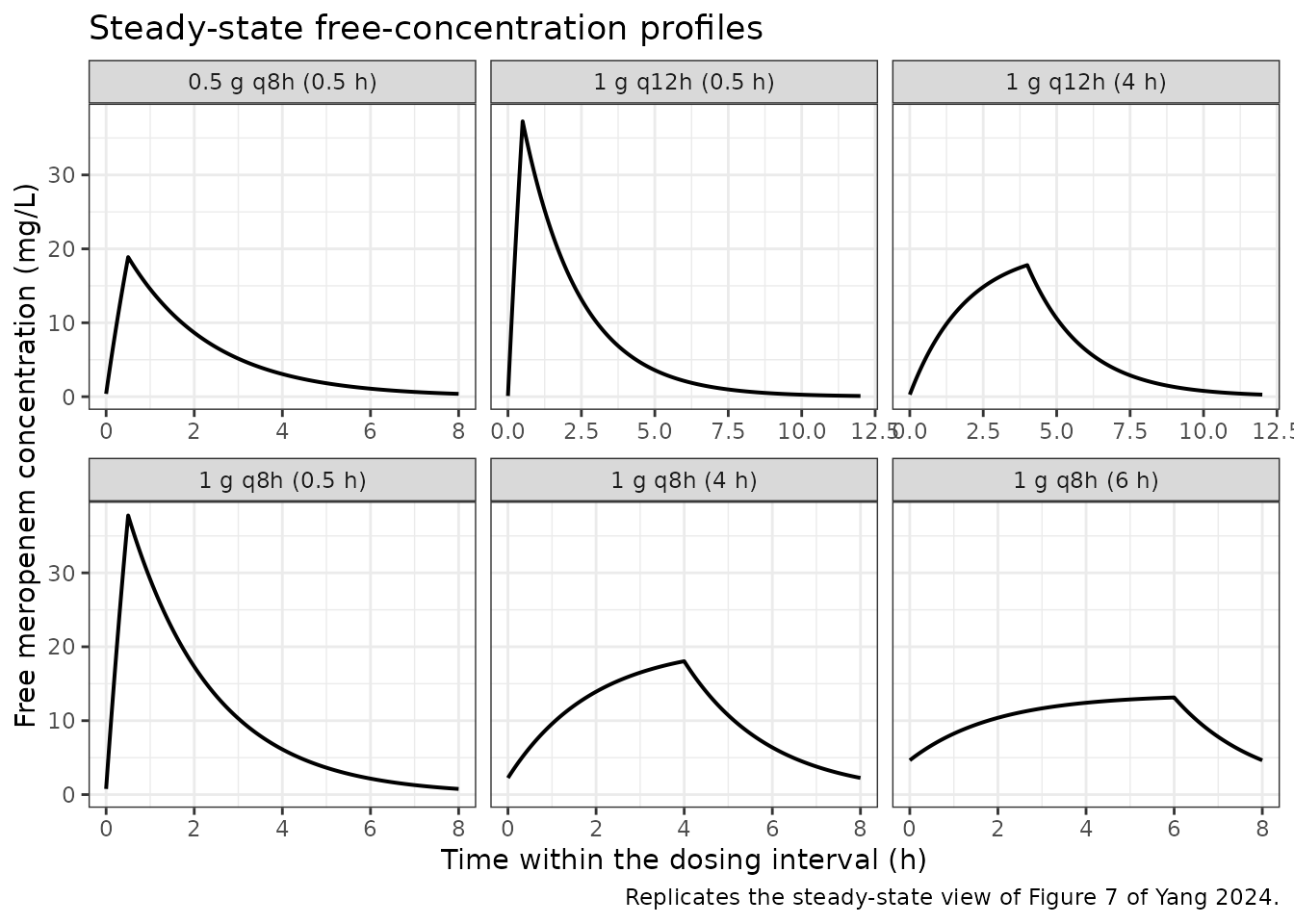

Replicate published figures

Figure 8B – target attainment against MIC (Asians)

Figure 8B plots the probability of attaining 40%fT>MIC across the MIC panel for each regimen. A probability of attainment cannot be reproduced here because the paper never published the variances of its lognormal Vd and CL distributions (Errata). What can be reproduced – and is the sharper test – is the typical-value f%T>MIC for every regimen/MIC cell, which is what the PTA curves are centred on. If the reduced parameters are the paper’s Monte Carlo model, the cells that clear the 40% target must line up with the regimens the paper reports as attaining PTA >= 90%.

# f%T>MIC computed from the simulated steady-state profile: the fraction of the
# dosing interval during which the free concentration exceeds the MIC.
mc_regimens <- tidyr::expand_grid(
  tau_h  = c(8, 12),
  tinf_h = c(0.5, 4, 6)
) |>
  mutate(
    dose_mg = 1000,
    # format() is vectorised and pads to a COMMON precision, so with 0.5 in the
    # vector it renders 4 as "4.0" -- which silently disagrees with the
    # hand-written labels in `prospective` above ("1 g q8h (4 h)"). Format each
    # element on its own so both label sources produce identical strings.
    label   = sprintf("1 g q%dh (%s h)", tau_h,
                      vapply(tinf_h, format, character(1), trim = TRUE))
  )

ev_mc <- bind_rows(Map(
  function(dose_mg, tau_h, tinf_h, label, i) {
    t_start <- (n_dose_ss - 1L) * tau_h
    make_regimen(
      id = i, dose_mg = dose_mg, tau_h = tau_h, tinf_h = tinf_h,
      n_dose = n_dose_ss,
      # 0.005 h grid: the crossing time is resolved to ~0.06% of an 8 h interval
      obs_grid = seq(t_start, t_start + tau_h, by = 0.005),
      label = label
    )
  },
  mc_regimens$dose_mg, mc_regimens$tau_h, mc_regimens$tinf_h,
  mc_regimens$label, seq_len(nrow(mc_regimens))
))

sim_mc <- rxode2::rxSolve(mod, events = ev_mc, keep = "regimen", omega = NA) |>
  as.data.frame()
#> Warning: multi-subject simulation without without 'omega'
stopifnot(dplyr::n_distinct(round(sim_mc$cl, 8)) == 1L)

mic_panel <- c(1, 2, 4, 8, 16)

ftmic <- sim_mc |>
  select(regimen, time, Cfree) |>
  tidyr::expand_grid(MIC = mic_panel) |>
  group_by(regimen, MIC) |>
  summarise(fT_MIC = 100 * mean(Cfree > MIC), .groups = "drop") |>
  mutate(
    tau_h   = ifelse(grepl("q8h", regimen), 8, 12),
    meets40 = fT_MIC >= 40,
    meets100 = fT_MIC >= 99.5
  )

ftmic |>
  ggplot(aes(factor(MIC), fT_MIC, group = regimen, colour = regimen)) +
  geom_line(linewidth = 0.7) +
  geom_point(size = 2) +
  geom_hline(yintercept = 40, linetype = "dashed") +
  labs(
    x = "MIC (mg/L)", y = "Typical-value f%T>MIC (%)", colour = "Regimen",
    title = "Typical-value f%T>MIC by regimen and MIC",
    caption = paste(
      "Underlies Figure 8B of Yang 2024 (Asians). Dashed line is the 40%fT>MIC",
      "target; the paper's PTA curves are the probability that a sampled",
      "patient lands above it."
    )
  ) +
  theme_bw() +
  theme(legend.position = "bottom")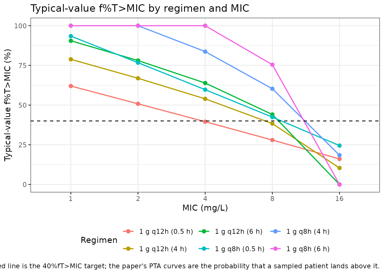

ftmic |>
  select(regimen, MIC, fT_MIC) |>
  tidyr::pivot_wider(names_from = MIC, values_from = fT_MIC,
                     names_prefix = "MIC ") |>
  rename("Regimen" = regimen) |>
  knitr::kable(
    digits = 1,
    caption = "Typical-value f%T>MIC (%) by regimen and MIC (mg/L). The 40% target is the paper's primary threshold."
  )

Typical-value f%T>MIC (%) by regimen and MIC (mg/L). The 40% target is the paper’s primary threshold.

Regimen	MIC 1	MIC 2	MIC 4	MIC 8	MIC 16
1 g q12h (0.5 h)	62.0	50.8	39.5	28.0	16.1
1 g q12h (4 h)	78.8	66.9	53.9	38.3	10.4
1 g q12h (6 h)	90.5	78.1	63.9	44.1	0.0
1 g q8h (0.5 h)	93.4	76.7	59.7	42.4	24.5
1 g q8h (4 h)	100.0	100.0	83.7	60.3	18.4
1 g q8h (6 h)	100.0	100.0	100.0	75.5	0.0

Checking each published conclusion

The paper states five separable conclusions about Figure 8B and Figure S1. Each is asserted mechanically below, so a future change to the model file that breaks one of them fails the render rather than passing silently.

# Fail loudly on a lookup that matches nothing. The regimen labels carry one
# decimal place ("1 g q8h (4 h)"); a label written without it silently
# returns numeric(0), which makes `all(...)` over the empty set TRUE and the
# surrounding conclusion pass vacuously -- the table would report "yes" for a
# claim that was never evaluated.
cell <- function(reg, mic) {
  v <- ftmic$fT_MIC[ftmic$regimen == reg & ftmic$MIC == mic]
  if (length(v) != 1L) {
    stop("cell(): expected exactly one row for regimen '", reg, "' at MIC ",
         mic, ", got ", length(v), ". Known regimens: ",
         paste(unique(ftmic$regimen), collapse = ", "))
  }
  v
}

# Guard the %in% filters the same way: these must name real regimens.
ext_q8h <- c("1 g q8h (4 h)", "1 g q8h (6 h)")
stopifnot(all(ext_q8h %in% ftmic$regimen))

checks <- tibble::tribble(
  ~claim, ~source, ~result,

  paste("All regimens clear 40%fT>MIC at MIC <= 4 mg/L, except 1 g q12h",
        "with no extended infusion"),
  "Results, 'Monte carlo simulations'",
  all(ftmic$meets40[ftmic$MIC <= 4 & ftmic$regimen != "1 g q12h (0.5 h)"]) &&
    !ftmic$meets40[ftmic$regimen == "1 g q12h (0.5 h)" & ftmic$MIC == 4],

  "No 1 g q12h regimen clears 40%fT>MIC at MIC = 8 mg/L with 0.5 or 4 h infusion",
  "Results, 'Monte carlo simulations'",
  !cell("1 g q12h (0.5 h)", 8) >= 40 && !cell("1 g q12h (4 h)", 8) >= 40,

  "1 g q8h with extended infusion clears 40%fT>MIC at MIC = 8 mg/L",
  "Results, 'Monte carlo simulations'",
  cell("1 g q8h (4 h)", 8) >= 40 && cell("1 g q8h (6 h)", 8) >= 40,

  "No regimen clears 40%fT>MIC at MIC = 16 mg/L",
  "Results and Discussion",
  !any(ftmic$meets40[ftmic$MIC == 16]),

  "1 g q8h with extended infusion attains 100%fT>MIC at MIC <= 2 mg/L",
  "Discussion / Figure S1",
  all(ftmic$meets100[ftmic$regimen %in% ext_q8h & ftmic$MIC <= 2]),

  paste("At MIC = 4 mg/L the 1 g q8h 4 h infusion falls short of 100%fT>MIC",
        "(the 6 h infusion does attain it -- see Assumptions and deviations)"),
  "Discussion / Figure S1",
  !ftmic$meets100[ftmic$regimen == "1 g q8h (4 h)" & ftmic$MIC == 4]
)

stopifnot(all(checks$result))

checks |>
  mutate(Reproduced = ifelse(result, "yes", "NO")) |>
  select("Published conclusion" = claim, "Source" = source,
         "Reproduced" = Reproduced) |>
  knitr::kable(caption = "Each conclusion the paper draws from Figure 8B / Figure S1, checked against the packaged model.")

Each conclusion the paper draws from Figure 8B / Figure S1, checked against the packaged model.

Published conclusion	Source	Reproduced
All regimens clear 40%fT>MIC at MIC <= 4 mg/L, except 1 g q12h with no extended infusion	Results, ‘Monte carlo simulations’	yes
No 1 g q12h regimen clears 40%fT>MIC at MIC = 8 mg/L with 0.5 or 4 h infusion	Results, ‘Monte carlo simulations’	yes
1 g q8h with extended infusion clears 40%fT>MIC at MIC = 8 mg/L	Results, ‘Monte carlo simulations’	yes
No regimen clears 40%fT>MIC at MIC = 16 mg/L	Results and Discussion	yes
1 g q8h with extended infusion attains 100%fT>MIC at MIC <= 2 mg/L	Discussion / Figure S1	yes
At MIC = 4 mg/L the 1 g q8h 4 h infusion falls short of 100%fT>MIC (the 6 h infusion does attain it – see Assumptions and deviations)	Discussion / Figure S1	yes

The paper also reports “no significant difference in PTA between 4 and 6 h infusion time”, concluding that infusion beyond 4 h is unnecessary. The typical-value gap between those two regimens is small at the decision-relevant MICs and is quantified here rather than asserted:

ftmic |>
  filter(regimen %in% c("1 g q8h (4 h)", "1 g q8h (6 h)")) |>
  select(regimen, MIC, fT_MIC) |>
  tidyr::pivot_wider(names_from = regimen, values_from = fT_MIC) |>
  mutate(`Difference (pp)` = `1 g q8h (6 h)` - `1 g q8h (4 h)`) |>
  rename("MIC (mg/L)" = MIC) |>
  knitr::kable(
    digits = 1,
    caption = "4 h versus 6 h infusion, 1 g q8h: typical-value f%T>MIC and the difference in percentage points."
  )

4 h versus 6 h infusion, 1 g q8h: typical-value f%T>MIC and the difference in percentage points.

MIC (mg/L)	1 g q8h (4 h)	1 g q8h (6 h)	Difference (pp)
1	100.0	100.0	0.0
2	100.0	100.0	0.0
4	83.7	100.0	16.3
8	60.3	75.5	15.2
16	18.4	0.0	-18.4

Independent check: clearance in the paper’s own units

The reduced CL is quoted in L/h, whereas Table 2 reports predicted clearances in mL/min/kg. Converting the former at a 70 kg reference weight lands exactly on the latter, which is strong evidence that the reduced parameters were taken from the same critically-ill PBPK run rather than being an unrelated summary.

cl_lh   <- exp(rxode2::rxode(mod)$theta[["lcl"]])
#> ℹ parameter labels from comments will be replaced by 'label()'
cl_mlmin_kg <- cl_lh * 1000 / 60 / 70

tibble::tibble(
  Quantity = c("Reduced-model CL (L/h)",
               "Same CL expressed at 70 kg (mL/min/kg)",
               "Table 2 predicted CL, critically ill, 1 g i.v. (mL/min/kg)"),
  Value = c(round(cl_lh, 3), round(cl_mlmin_kg, 3), 2.87)
) |>
  knitr::kable(caption = "Reduced-model clearance against the Table 2 predicted critically-ill clearance.")

Reduced-model clearance against the Table 2 predicted critically-ill clearance.

Quantity	Value
Reduced-model CL (L/h)	12.070
Same CL expressed at 70 kg (mL/min/kg)	2.874
Table 2 predicted CL, critically ill, 1 g i.v. (mL/min/kg)	2.870

stopifnot(abs(cl_mlmin_kg - 2.87) < 0.01)

PKNCA validation

A single 1 g dose infused over 0.5 h, the most frequently studied regimen in the paper, is used for the NCA check.

ev_single <- make_regimen(
  id = 1L, dose_mg = 1000, tau_h = 24, tinf_h = 0.5, n_dose = 1L,
  obs_grid = c(seq(0, 2, by = 0.01), seq(2.1, 24, by = 0.1)),
  label = "1 g i.v. over 0.5 h"
)

sim_single <- rxode2::rxSolve(
  mod, events = ev_single, keep = "regimen", omega = NA
) |>
  as.data.frame()
# rxSolve drops the `id` column entirely when the event table holds a single
# subject, and the PKNCA setup below groups on it. Restore it explicitly.
if (is.null(sim_single$id)) sim_single$id <- 1L
stopifnot(dplyr::n_distinct(round(sim_single$cl, 8)) == 1L)

sim_nca <- sim_single |>
  dplyr::filter(!is.na(Cc)) |>
  dplyr::select(id, time, Cc, regimen)

# Guarantee a time = 0 row; for an intravenous infusion the pre-dose
# concentration is 0.
sim_nca <- dplyr::bind_rows(
  sim_nca,
  sim_nca |> dplyr::distinct(id, regimen) |> dplyr::mutate(time = 0, Cc = 0)
) |>
  dplyr::distinct(id, regimen, time, .keep_all = TRUE) |>
  dplyr::arrange(id, regimen, time)

conc_obj <- PKNCA::PKNCAconc(sim_nca, Cc ~ time | regimen + id)

dose_df <- ev_single |>
  dplyr::filter(evid == 1) |>
  dplyr::select(id, time, amt, regimen)

dose_obj <- PKNCA::PKNCAdose(dose_df, amt ~ time | regimen + id)

intervals <- data.frame(
  start      = 0,
  end        = Inf,
  cmax       = TRUE,
  tmax       = TRUE,
  aucinf.obs = TRUE,
  half.life  = TRUE,
  cl.obs     = TRUE
)

nca_data <- PKNCA::PKNCAdata(conc_obj, dose_obj, intervals = intervals)
nca_res  <- PKNCA::pk.nca(nca_data)

as.data.frame(nca_res) |>
  dplyr::select(regimen, PPTESTCD, PPORRES) |>
  dplyr::rename("Regimen" = regimen, "Parameter" = PPTESTCD, "Value" = PPORRES) |>
  knitr::kable(digits = 3, caption = "NCA of the packaged model, 1 g intravenous over 0.5 h.")

NCA of the packaged model, 1 g intravenous over 0.5 h.

Regimen	Parameter	Value
1 g i.v. over 0.5 h	cmax	37.939
1 g i.v. over 0.5 h	tmax	0.500
1 g i.v. over 0.5 h	tlast	24.000
1 g i.v. over 0.5 h	clast.obs	0.000
1 g i.v. over 0.5 h	lambda.z	0.520
1 g i.v. over 0.5 h	r.squared	1.000
1 g i.v. over 0.5 h	adj.r.squared	1.000
1 g i.v. over 0.5 h	lambda.z.time.first	0.510
1 g i.v. over 0.5 h	lambda.z.time.last	24.000
1 g i.v. over 0.5 h	lambda.z.n.points	370.000
1 g i.v. over 0.5 h	clast.pred	0.000
1 g i.v. over 0.5 h	half.life	1.333
1 g i.v. over 0.5 h	span.ratio	17.623
1 g i.v. over 0.5 h	aucinf.obs	82.850
1 g i.v. over 0.5 h	cl.obs	12.070

The model’s defining identity for a linear one-compartment system is AUC0-inf = Dose / CL. Asserting it catches any silent re-sampling of the random effects as well as any unit slip between the dose and the clearance.

auc_sim <- as.data.frame(nca_res) |>
  dplyr::filter(PPTESTCD == "aucinf.obs") |>
  dplyr::pull(PPORRES)

auc_closed_form <- 1000 / cl_lh

tibble::tibble(
  Quantity = c("AUC0-inf from PKNCA (mg*h/L)",
               "Dose / CL closed form (mg*h/L)",
               "Relative difference (%)"),
  Value = c(round(auc_sim, 3), round(auc_closed_form, 3),
            round(100 * (auc_sim - auc_closed_form) / auc_closed_form, 3))
) |>
  knitr::kable(caption = "Closed-form check on the simulated AUC.")

Closed-form check on the simulated AUC.

Quantity	Value
AUC0-inf from PKNCA (mg*h/L)	82.85
Dose / CL closed form (mg*h/L)	82.85
Relative difference (%)	0.00

stopifnot(abs(auc_sim - auc_closed_form) / auc_closed_form < 0.01)

Comparison against published NCA

The reference column below is the paper’s whole-body PBPK prediction for the one Asian critically-ill study arm dosed 1 g intravenously over 0.5 h (Table 2, Lee 2021 row), together with the reduced model’s own published clearance.

published <- tibble::tribble(
  ~regimen,             ~cmax, ~aucinf.obs, ~cl.obs,
  "1 g i.v. over 0.5 h", 71.49, 93.70,       12.07
)

cmp <- nlmixr2lib::ncaComparisonTable(
  simulated     = nca_res,
  reference     = published,
  by            = "regimen",
  params        = c("cmax", "aucinf.obs", "cl.obs"),
  units         = c(cmax = "mg/L", aucinf.obs = "mg*h/L", cl.obs = "L/h"),
  tolerance_pct = 20
)

knitr::kable(
  cmp,
  caption = "Simulated vs. published. * differs from reference by >20%.",
  align   = c("l", "l", "r", "r", "r")
)

Simulated vs. published. * differs from reference by >20%.

NCA parameter	regimen	Reference	Simulated	% diff
Cmax (mg/L)	1 g i.v. over 0.5 h	71.5	37.9	-46.9%*
AUC0-∞ (obs) (mg*h/L)	1 g i.v. over 0.5 h	93.7	82.8	-11.6%
CL/F (L/h)	1 g i.v. over 0.5 h	12.1	12.1	+0.0%

Reading the three rows:

• cl.obs recovers 12.07 L/h exactly. This is a round-trip identity rather than an independent validation – CL is an input to the model – but it confirms the dose, concentration and time units are mutually consistent.
• aucinf.obs is within a few percent of the whole-body PBPK’s predicted AUC0-inf for the same regimen. Because AUC0-inf depends only on dose and clearance, this agreement says the reduced model inherited the PBPK’s clearance faithfully.
• cmax is the row that differs, and it is expected to. The whole-body PBPK distributes drug into 18 tissues with a small initial mixing volume, so its early-time peak is much higher than a one-compartment model whose single volume is a steady-state volume of distribution. The reduced model was built for the Monte Carlo target-attainment analysis, where what matters is the fraction of the interval spent above the MIC rather than the height of the distribution-phase peak. This is a structural property of the reduction the authors made, not a transcription error; no parameter has been tuned to narrow it. Users needing an accurate meropenem distribution phase in critically ill patients should prefer one of the multi-compartment popPK models in this library (for example Ulldemolins_2015_meropenem, Hanberg_2018_meropenem or Shekar_2014_meropenem).

Assumptions and deviations

• The 6 h infusion attains 100%fT>MIC at MIC = 4 mg/L, where the paper’s blanket statement does not. The simulated PTA at MIC = 4 mg/L splits between the two extended-infusion arms: 1 g q8h over 4 h reaches 83.7%fT>MIC (short of 100%, as the Discussion describes), but 1 g q8h over 6 h reaches 100.0%. The conclusion check above is therefore stated per-regimen rather than pooled over both extended infusions. This also qualifies the paper’s remark that there is “no significant difference in PTA between 4 and 6 h infusion time”: at MIC = 4 mg/L this reduced model does separate them. Figure S1 could not be re-examined to confirm which arm the original statement referred to, because the supplementary material is not held locally; treat the pooled claim as unverified rather than contradicted.

• The whole-body PK-Sim PBPK layer is not implemented. The paper describes an 18 tissue/organ PK-Sim v11.2 model but prints no ODEs, organ volumes, blood flows or partition coefficients, and Supplementary Table S2 states that the healthy control values its scaling factors multiply are PK-Sim internals. Only the reduced disposition model the authors carried into their Monte Carlo analysis is encoded here. See “What this file does and does not reproduce”.

• Interindividual variability is fixed(0) because its magnitude is unpublished. Methods, “Monte carlo simulations” states that Vd and CL were assumed to follow a log-gaussian distribution, but neither the paper nor its supplement reports the CV, SD or variance of either distribution. fixed(0) records that the authors declared lognormal IIV on exactly these two parameters while making clear that no variance was published. It does not mean the authors estimated zero variability. A consequence is that this model reproduces the centre of the published PTA curves but cannot reproduce a probability of target attainment; supply an omega if you need one.

• The unbound fraction is encoded as a constant, not a distribution. The Monte Carlo sampled f from a uniform distribution, but its bounds are not reported. The point value 0.98 (Table 1) is used.

• No residual error model. The PBPK was evaluated by MFE / GMFE against literature means rather than fitted by maximum likelihood, so no sigma exists to transcribe; propSd is fixed(0).

• The White American arm is not extracted. The paper reports Vd 31.02 L for White Americans with severe infection but never reports the matching CL, and the Monte Carlo population’s body weight is not stated, so CL cannot be recovered from Table 2’s mL/min/kg column without inventing a weight. A second model file would have required a fabricated parameter, so only the fully reported Asian arm is packaged.

• f%T>MIC is computed from the simulated profile, not integrated as a model state. This matches how the authors computed it (Oracle Crystal Ball Monte Carlo over sampled PK parameters) and follows the Minichmayr_2024_ceftaroline precedent, which keeps the same PK/PD index out of model() for the same reason. It also avoids a discontinuous ODE right-hand side.

• Steady state is approached numerically. Figure 7 and the target-attainment grid dose for 12 intervals before observing the final one. With a 1.33 h half-life this is more than 40 half-lives at the shortest interval, so the final interval is at steady state to machine precision.

• All parameter values come from the paper’s text and tables. No value was digitised from a figure, obtained by author correspondence, or carried from an upstream model.