Indomethacin exposure-response in preterm neonates (Yeung 2025)
Source:vignettes/articles/Yeung_2025_indomethacin.Rmd
Yeung_2025_indomethacin.RmdModel and source
- Citation: Yeung CHT, Sekulich DC, Scott A, Nolte WM, Gibson K, Su R, Alrifai MW, Lopata SM, Lewis T, Reese J, Maharaj A (2025). The Relationship of Indomethacin Exposure With Efficacy and Renal Toxicity Outcomes for Preterm Infants in the Neonatal Intensive Care Unit. Clin Transl Sci 18(5):e70251. doi:10.1111/cts.70251.
- Article: https://doi.org/10.1111/cts.70251
- Structural PK model: Krzyzanski W et al. (2023), https://doi.org/10.1002/psp4.12881
Yeung 2025 relates model-predicted indomethacin exposure to three outcomes in preterm neonates from two US neonatal intensive care units: prevention of severe intraventricular hemorrhage (IVH), closure of a patent ductus arteriosus (PDA), and renal toxicity measured as the urine output (UOP) rate nadir within 12 h of a dose. Exposure came from the indomethacin population PK (IND popPK) model of Krzyzanski 2023 with its CYP2C9 genotype covariate removed, re-estimated separately on each site’s data (supplement Table S2). The paper contributes five models, packaged as five files:
| Model | What it is |
|---|---|
Yeung_2025_indomethacin_cmh |
CYP2C9-reduced popPK, re-estimated on the Children’s Mercy Hospital (CMH) dataset (plasma, dried blood spot and urine) |
Yeung_2025_indomethacin_vumc |
CYP2C9-reduced popPK, re-estimated on the Vanderbilt (VUMC) dried-blood-spot dataset |
Yeung_2025_indomethacin_ivh |
Logistic regression for severe IVH (Table 2) |
Yeung_2025_indomethacin_pda |
Mixed-effects logistic regression for PDA treatment failure (Table 2) |
Yeung_2025_indomethacin_uop |
Linear mixed-effects model for the ln UOP rate nadir (Table 2, Figure 4) |
The three regressions take exposure as a covariate column
(AUC_INDO, AUC_INDO_COURSE,
CMAX); the two PK models are how that column is
produced.
Population
Eighty-three neonates contributed (Yeung 2025 Table 1). The CMH
cohort (45 infants given 0.1 mg/kg IV q24h x3 for IVH prophylaxis, 18
treated for PDA with 0.1 mg/kg q12h x3 per course, 10 in both) had a
median weight of 760 g and gestational age of 26.1 weeks for the IVH
group. The VUMC cohort (30 infants, < 28 weeks and < 1000 g)
received a single 0.2 mg/kg dose at about 12 h of life; median weight
645 g, gestational age 24.9 weeks. Renal toxicity was measured at CMH
only. Per-model details are in each file’s population
metadata, e.g.
readModelDb("Yeung_2025_indomethacin_vumc")()$population.
Source trace
| Equation / parameter | Value | Source location |
|---|---|---|
One-compartment IV bolus; d/dt(urine) = CLR * Cc
|
– | Krzyzanski 2023 Equations 1-3 (structure retained by Yeung 2025 Methods ‘PopPK Modeling’) |
| Power PNA effect, centred on 1.25 days | – | Krzyzanski 2023 Equation 5 and Results (‘PNAmean = 1.25 days’) |
| Log-scale residual, separate DBS variance | – | Krzyzanski 2023 Equations 7-8 |
| CMH: V, CLR, CLH | 0.435 L, 0.0000172 L/h, 0.000647 L/h | Table S2, CMH column |
| CMH: PNA exponents on CLR, CLH | -0.192, 0.901 | Table S2, CMH column |
| CMH: IIV V, CLR, CLH | 38.5%, 69.0%, 215.4% | Table S2 (IIV% = 100 sqrt(exp(omega^2) - 1)) |
| CMH: residual variances plasma, DBS, urine | 0.0978, 0.272, 0.0964 | Table S2 |
| VUMC: V, CLH, PNA exponent on CLH | 0.164 L, 0.000572 L/h, 1.21 | Table S2, VUMC column |
| VUMC: IIV V, CLH; DBS residual variance | 26.3%, 69.8%; 0.181 | Table S2, VUMC column |
| VUMC: renal, plasma and urine terms | fixed at CMH values | Table S2 footnote (‘fixing all renal clearance … and urine terms’) |
| IVH logit: intercept, AUC, site, GA, PNA, sex, race | 14.5, -0.0005, -1.79, -0.66, 0.087, -0.78, +0.91 | Table 2, IVH block (race sign: see Assumptions) |
| PDA logit: intercept, AUCcourse, GA, PNA, condition, sex, race | 2.79, -0.0065, -0.23, 0.009, 0.24, 2.35, 0.99 | Table 2, PDA block |
| ln UOP nadir: intercept, Cmax | 1.23, -0.088 | Table 2, UOP block |
| ln UOP nadir: fluid intake | 0.0034 per mL/kg/day | Table 2, UOP block (see Assumptions) |
| ln UOP nadir: total SD | 0.53 | Back-solved from the Results text (see the Figure 4 section) |
PK models: individual exposure
Postnatal age (PNA) is time-varying in both PK models, so the event table carries PNA on every record. Doses are absolute amounts (mg/kg times weight). Each cohort uses the site’s median weight and postnatal age at the first dose (Table 1) with 200 simulated infants.
make_cohort <- function(n, wt, pna0_h, dose_mgkg, n_dose, tau, site, id0 = 0) {
  obs_t <- sort(unique(c(seq(0, 24, by = 0.5), seq(24, 504, by = 4))))
  dose_t <- (seq_len(n_dose) - 1) * tau
  one <- bind_rows(
    data.frame(time = dose_t, evid = 1, amt = dose_mgkg * wt),
    data.frame(time = obs_t, evid = 0, amt = 0)
  ) |>
    arrange(time, desc(evid))
  tidyr::expand_grid(id = id0 + seq_len(n), one) |>
    mutate(
      cmt = "central",
      # The models have two endpoints (Cc, Aurine); dvid = 1 selects Cc.
      dvid = ifelse(evid == 0, 1L, NA_integer_),
      PNA = (pna0_h + time) / 24 / 30.4375,
      SAMPLE_DBS = 0,
      site = site,
      dose_course = dose_mgkg * n_dose
    )
}

ev_cmh <- make_cohort(200, wt = 0.760, pna0_h = 5.5, dose_mgkg = 0.1,
                      n_dose = 3, tau = 24, site = "CMH")
ev_vumc <- make_cohort(200, wt = 0.645, pna0_h = 13, dose_mgkg = 0.2,
                       n_dose = 1, tau = 24, site = "VUMC", id0 = 1000)

mod_cmh <- readModelDb("Yeung_2025_indomethacin_cmh")
mod_vumc <- readModelDb("Yeung_2025_indomethacin_vumc")

rxode2::rxSetSeed(20251)
sim_cmh <- rxSolve(mod_cmh, ev_cmh, returnType = "data.frame",
                   keep = c("site", "dose_course"))
sim_vumc <- rxSolve(mod_vumc, ev_vumc, returnType = "data.frame",
                    keep = c("site", "dose_course"))
sim_pk <- bind_rows(sim_cmh, sim_vumc)

typ_cmh <- rxSolve(rxode2::zeroRe(mod_cmh), filter(ev_cmh, id == 1),
                   returnType = "data.frame", keep = "site")
typ_vumc <- rxSolve(rxode2::zeroRe(mod_vumc), filter(ev_vumc, id == 1001),
                    returnType = "data.frame", keep = "site")
typ_pk <- bind_rows(typ_cmh, typ_vumc)
pk_band <- sim_pk |>
  filter(time <= 168) |>
  group_by(site, time) |>
  summarise(
    lo = quantile(Cc, 0.05), med = median(Cc), hi = quantile(Cc, 0.95),
    .groups = "drop"
  )
ggplot(pk_band, aes(time, med)) +
  geom_ribbon(aes(ymin = lo, ymax = hi), alpha = 0.25) +
  geom_line() +
  geom_line(data = filter(typ_pk, time <= 168), aes(y = Cc), linetype = 2) +
  facet_wrap(~site) +
  labs(x = "Time after first dose (h)", y = "Indomethacin plasma (ug/mL)",
       caption = paste("Median and 90% interval of 200 simulated infants per",
                       "site; dashed = typical value."))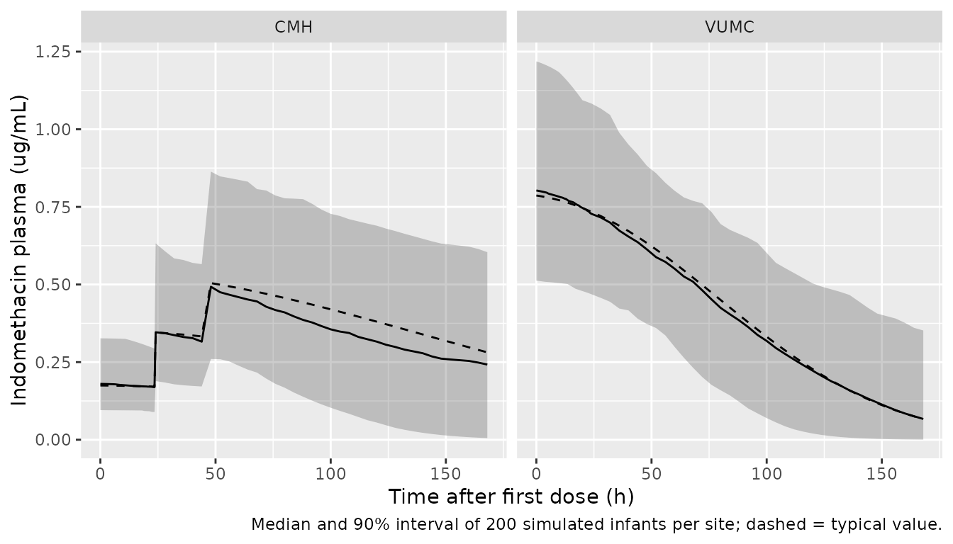
Dose-normalised AUC0-inf (Figure 2)
Yeung 2025 Figure 2 plots the popPK-predicted AUC0-inf divided by the total course dose (0.3 mg/kg at CMH, 0.2 mg/kg at VUMC). The medians read from the figure are about 230 (CMH) and 360 (VUMC) ug*h/mL per mg/kg, pooling the two outcome groups at each site.
conc_obj <- PKNCAconc(
  sim_pk |> filter(!is.na(Cc)) |> select(id, time, Cc, site),
  Cc ~ time | site + id
)
dose_obj <- PKNCAdose(
  bind_rows(ev_cmh, ev_vumc) |> filter(evid == 1) |>
    select(id, time, amt, site),
  amt ~ time | site + id
)
intervals <- data.frame(start = 0, end = Inf, aucinf.obs = TRUE, cmax = TRUE,
                        half.life = TRUE)
nca_res <- pk.nca(PKNCAdata(conc_obj, dose_obj, intervals = intervals))

course_dose <- bind_rows(ev_cmh, ev_vumc) |> distinct(id, dose_course)
auc_dn <- as.data.frame(nca_res) |>
  filter(PPTESTCD == "aucinf.obs") |>
  left_join(course_dose, by = "id") |>
  mutate(PPORRES = PPORRES / dose_course)

reference_fig2 <- data.frame(site = c("CMH", "VUMC"),
                             aucinf.obs = c(230, 360))
tbl <- ncaComparisonTable(
  auc_dn |> select(site, PPTESTCD, PPORRES),
  reference_fig2,
  by = "site",
  units = c(aucinf.obs = "ug*h/mL per mg/kg")
)
knitr::kable(tbl, caption = paste("Simulated vs Figure 2 median",
"dose-normalised AUC0-inf."))| NCA parameter | site | Reference | Simulated | % diff |
|---|---|---|---|---|
| AUC0-∞ (obs) (ug*h/mL per mg/kg) | CMH | 230 | 305 | +32.7%* |
| AUC0-∞ (obs) (ug*h/mL per mg/kg) | VUMC | 360 | 378 | +5.0% |
med_dn <- auc_dn |> group_by(site) |> summarise(med = median(PPORRES))
ratio <- med_dn$med / reference_fig2$aucinf.obs[match(med_dn$site, reference_fig2$site)]
ratio
#> [1] 1.327474 1.049526
# A transcription error in V or CLH (units, a dropped digit) moves the median
# several-fold; the band allows for cohort covariates fixed at site medians
# and for reading medians off a figure.
stopifnot(all(ratio > 0.67), all(ratio < 1.5))
The VUMC median reproduces the figure closely. The CMH median is higher than the figure because the simulation gives every infant the median postnatal age at first dose (5.5 h) and the nominal 0.1 mg/kg dose, while the real cohort spans 0.23-53.7 h and 0.085-0.40 mg/kg; older infants clear the drug faster and pull the observed median down.
Clearance matures quickly with postnatal age (exponent 0.901 at CMH, 1.21 at VUMC), so elimination accelerates over the profile. At the CMH centring age of 1.25 days the typical half-life is ln(2) x 0.435 / (0.0000172 + 0.000647) = 454 h, while the terminal half-life PKNCA estimates from the last days of the three-week window, when the infants are weeks old, is far shorter:
as.data.frame(nca_res) |>
  filter(PPTESTCD == "half.life") |>
  group_by(site) |>
  summarise(median_half_life_h = median(PPORRES, na.rm = TRUE)) |>
knitr::kable(digits = 1)| site | median_half_life_h |
|---|---|
| CMH | 40.6 |
| VUMC | 7.7 |
Severe IVH (Table 2, Table 3)
The IVH logistic model as printed in Table 2 includes all six screened covariates. Only gestational age is significant (odds ratio 0.517 per week). The figure below shows the predicted probability of severe IVH across gestational age for a male, Black CMH infant at a dose-normalised AUC of 230 and a postnatal age at first dose of 5.5 h, with the observed proportions of Table 3 (“our study with indomethacin”) for reference.
# The regression models carry no between-subject variance (none, or a
# zero-variance random intercept), so rxode2's warning that a multi-subject
# solve has no omega is expected here and in the PDA and UOP chunks.
mod_ivh <- readModelDb("Yeung_2025_indomethacin_ivh")
ga_grid <- seq(23, 30, by = 0.25)
ivh_dat <- data.frame(
  id = seq_along(ga_grid), time = 0, evid = 0, GA = ga_grid,
  AUC_INDO = 230, STUDY_VUMC = 0, PNA = 5.5 / 24 / 30.4375,
  SEXF = 0, RACE_BLACK = 1
)
ivh_pred <- rxSolve(mod_ivh, ivh_dat, returnType = "data.frame")

# Closed-form check: the model's per-week odds ratio equals exp(-0.66).
odds <- with(ivh_pred, prob_ivh_severe / (1 - prob_ivh_severe))
or_week <- odds[ga_grid == 27] / odds[ga_grid == 26]
stopifnot(abs(or_week - exp(-0.66)) < 1e-6)

tab3 <- data.frame(GA = c(23.5, 25.5, 27.5, 29.5),
                   observed = c(2 / 13, 5 / 32, 2 / 24, 0 / 6))
ggplot(ivh_pred, aes(GA, prob_ivh_severe)) +
  geom_line() +
  geom_point(data = tab3, aes(GA, observed), shape = 1, size = 3) +
  labs(x = "Gestational age (weeks)", y = "P(severe IVH)",
       caption = "Line: Table 2 model. Circles: Table 3 observed proportions.")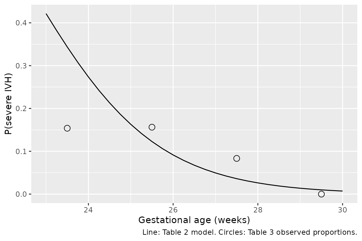
Table 3’s “probability of increased severity” column comes from a refit with gestational age as the only covariate, whose intercept and slope are not printed, so it is not reproduced here.
PDA treatment failure (Table 2)
No covariate in the PDA model is significant. The subject random intercept’s variance is not reported, so it is held at zero and the model returns the population-average logit. The predicted probability over the AUCcourse range of Figure 3, for a male, Black infant of 26 weeks gestational age at a postnatal age of 11 days without prior IVH prophylaxis:
mod_pda <- readModelDb("Yeung_2025_indomethacin_pda")
auc_grid <- seq(0, 170, by = 5)
pda_dat <- data.frame(
  id = seq_along(auc_grid), time = 0, evid = 0, AUC_INDO_COURSE = auc_grid,
  GA = 26, PNA = 11 / 30.4375, PRIOR_INDO = 0, SEXF = 0, RACE_BLACK = 1
)
pda_pred <- rxSolve(mod_pda, pda_dat, returnType = "data.frame")
stopifnot(abs(diff(range(qlogis(pda_pred$prob_pda_failure))) -
                0.0065 * 170) < 1e-6)
ggplot(pda_pred, aes(AUC_INDO_COURSE, prob_pda_failure)) +
  geom_line() +
  labs(x = "AUCcourse (ug*h/mL)", y = "P(PDA treatment failure)")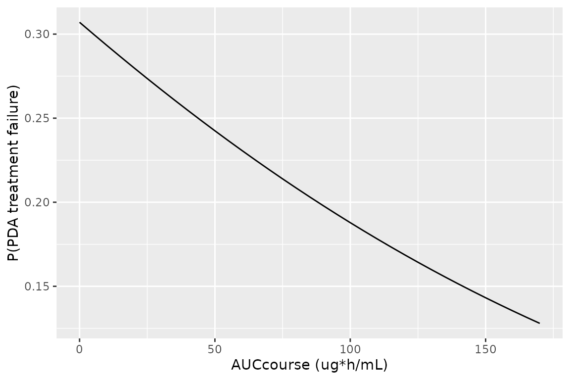
Renal toxicity (Figure 4)
Yeung 2025 simulated 1000 infants at each Cmax from 0 to 30 ug/mL with the fluid-intake covariate at its median, including between-subject and residual variability, and reported that the median UOP nadir falls below 1 and 0.5 mL/kg/h at Cmax 14 and 22 ug/mL, and the 5th percentile at 5 and 12 ug/mL. Neither variance of the mixed model is printed. A single draw per simulated infant depends only on their sum, and the four printed 5th-percentile crossings bound its square root to 0.527-0.534 on the ln scale; the model carries 0.53, all in the residual term. Figure 4’s 90% band is about +/- 0.85 around the median on the ln scale, i.e. 1.645 x 0.52, consistent with this.
mod_uop <- readModelDb("Yeung_2025_indomethacin_uop")
cmax_grid <- 0:30
uop_dat <- tidyr::expand_grid(cmax = cmax_grid, rep = 1:200) |>
  mutate(id = row_number(), time = 0, evid = 0, CMAX = cmax,
         WT = 0.8, FLUID_IN_24H = 150 * 0.8) |>
  select(id, time, evid, CMAX, WT, FLUID_IN_24H)
rxode2::rxSetSeed(20254)
uop_sim <- rxSolve(mod_uop, uop_dat, returnType = "data.frame")

uop_sum <- uop_sim |>
  group_by(CMAX) |>
  summarise(med = median(sim), p05 = quantile(sim, 0.05),
            p95 = quantile(sim, 0.95), .groups = "drop")
uop_typ <- rxSolve(rxode2::zeroRe(mod_uop),
                   uop_dat |> distinct(CMAX, .keep_all = TRUE),
                   returnType = "data.frame")
ggplot(uop_sum, aes(CMAX)) +
  geom_line(aes(y = log(p05)), colour = "firebrick") +
  geom_line(aes(y = log(p95)), colour = "firebrick") +
  geom_line(data = uop_typ, aes(y = log(urine_output_nadir)),
            colour = "steelblue") +
  geom_hline(yintercept = 0, linetype = 2) +
  geom_hline(yintercept = log(0.5), linetype = 3) +
  labs(x = "Cmax per dose (ug/mL)", y = "ln UOP rate nadir within 12 h",
       caption = paste("Replicates Figure 4 of Yeung 2025: median (blue) and",
                       "5th/95th percentiles (red) of 200 simulated infants per",
                       "Cmax; dashed 1 and dotted 0.5 mL/kg/h."))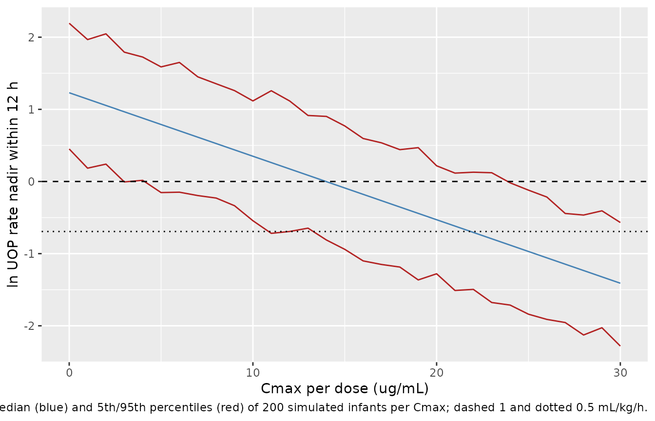
The threshold crossings come from the model’s own parameters in closed form (the median is the typical value; the 5th percentile shifts it by qnorm(0.05) x 0.53):
p <- rxode2::rxode(mod_uop)$theta
med_ln <- p[["lurine_output_nadir"]] + p[["e_cmax_urine_output_nadir"]] * cmax_grid
p05_ln <- med_ln + qnorm(0.05) * p[["expSd_urine_output_nadir"]]
crossings <- c(
  median_below_1 = min(cmax_grid[med_ln < 0]),
  median_below_0.5 = min(cmax_grid[med_ln < log(0.5)]),
  p05_below_1 = min(cmax_grid[p05_ln < 0]),
  p05_below_0.5 = min(cmax_grid[p05_ln < log(0.5)])
)
crossings
#>   median_below_1 median_below_0.5      p05_below_1    p05_below_0.5
#>               14               22                5               12
stopifnot(identical(unname(crossings), c(14L, 22L, 5L, 12L)))
# 8.4% lower nadir per 1 ug/mL (Results).
stopifnot(abs((1 - exp(p[["e_cmax_urine_output_nadir"]])) * 100 - 8.4) < 0.05)
The two median crossings test the printed intercept and Cmax slope independently of the variability; the two 5th-percentile crossings only confirm the back-solved SD.
The model-predicted per-dose Cmax in the simulated CMH cohort sits in the same low range as the observed points of Figure 4 (almost all below 5 ug/mL), far from the toxic thresholds:
as.data.frame(nca_res) |>
  filter(PPTESTCD == "cmax") |>
  group_by(site) |>
  summarise(median = median(PPORRES), p95 = quantile(PPORRES, 0.95)) |>
knitr::kable(digits = 2, caption = "Simulated Cmax (ug/mL) over the course.")| site | median | p95 |
|---|---|---|
| CMH | 0.49 | 0.86 |
| VUMC | 0.80 | 1.22 |
Assumptions and deviations
-
Two Table 2 cells contradict their own confidence
intervals. Every other row of Table 2 has its estimate inside
its 95% CI and a p-value consistent with the CI width, so each defect is
isolated to one cell.
- Race in the IVH model is printed -0.91 with 95% CI (-0.67, 2.74). The CI excludes the estimate; it is consistent with +0.91 (mildly skewed profile interval, Wald p about 0.29 against the printed 0.28). The model uses +0.91 (non-Black vs Black). Correcting the CI instead would need two cells changed and their order swapped.
-
Fluid intake in the renal model is printed 0.00034
(mL/kg/h) with 95% CI (0.00068, 0.0061) and p = 0.014. The CI midpoint
is 0.0034, and 0.0034 with the CI half-width gives z = 2.46, p = 0.014,
matching the printed p; keeping 0.00034 would need both CI bounds wrong.
The unit is taken as mL/kg/day: Methods define the covariate as the
weight-normalised fluid volume over the 24 h after the dose, Table 1
reports that intake in mL/kg/day (median 150, range 64.5-227.7), and
only that scale gives a standard error of the observed size for a
covariate spread of a few tens of units. The model forms the covariate
as
FLUID_IN_24H / WT - 150. At the median intake it is zero, so Figure 4 does not depend on it.
- Variance of the renal model. Not printed; 0.53 is the total SD back-solved from the Results text (see the Figure 4 section). The subject random intercept is held at zero and all variability is residual, which is exact for one observation per infant but ignores within-infant correlation across doses.
- PDA random intercept variance is not reported; held at zero.
- IVH and PDA models are as printed in Table 2. Methods describe backward stepwise selection, so the tabulated coefficients are the multivariable fits before non-significant covariates were removed. The reduced IVH model (gestational age only) used for Table 3 is not printed. The Results text quotes the gestational-age slope as -0.67 while Table 2 prints -0.66; the table value is used.
-
VUMC renal, plasma and urine terms. Table S2 prints
NA for them and the footnote says they were held fixed; they are carried
at the CMH re-estimate values (renal clearance and its PNA exponent and
IIV, plasma and urine residual variances) and marked
fixed(). The footnote also lists “dried blood spot terms” as fixed while printing an estimated DBS residual variance (0.181, RSE 23.9%); the estimate is used. - PNA centring. Yeung 2025 retained the Krzyzanski 2023 structure without restating the centring value; 1.25 days (the development cohort’s mean postnatal age at first dose) is used for both re-estimates.
- CMH subject count. The popPK re-estimate used the CMH development dataset, whose size Yeung 2025 does not restate; the CMH file records the 38 infants of the Krzyzanski 2023 development cohort.
- Exposure provenance. The PDA AUCcourse and renal Cmax were derived in the paper from the full IND popPK model with the CYP2C9 covariate (Krzyzanski 2023), not from either CYP2C9-reduced model here.
- Simulation cohorts use each site’s median weight and postnatal age at first dose, nominal doses and plasma sampling.