Oseltamivir influenza-pandemic SEIR model (Kamal 2017)
Source:vignettes/articles/Kamal_2017_oseltamivir.Rmd
Kamal_2017_oseltamivir.RmdModel and source
- Citation: Kamal MA, Smith PF, Chaiyakunapruk N, Wu DBC, Pratoomsoot C, Lee KKC, Chong HY, Nelson RE, Nieforth K, Dall G, Toovey S, Kong DCM, Kamauu A, Kirkpatrick CM, Rayner CR. Interdisciplinary pharmacometrics linking oseltamivir pharmacology, influenza epidemiology and health economics to inform antiviral use in pandemics. Br J Clin Pharmacol. 2017;83(7):1580-1594. doi:10.1111/bcp.13229. The oseltamivir carboxylate exposures behind f_auchigh come from Kamal MA, Van Wart SA, Rayner CR, Subramoney V, Reynolds DK, Bulik CC, et al. Population pharmacokinetics of oseltamivir: pediatrics through geriatrics. Antimicrob Agents Chemother. 2013;57(7):3470-3477; see modellib(‘Kamal_2013_oseltamivir’). The AUC breakpoint and the Tshed distributions come from Rayner CR, Bulik CC, Kamal MA, Reynolds DK, Toovey S, Hammel JP, et al. Pharmacokinetic-pharmacodynamic determinants of oseltamivir efficacy using data from phase 2 inoculation studies. Antimicrob Agents Chemother. 2013;57(7):3478-3487.
- Description: QSP. Population-level influenza transmission model (stochastic SEIR) linked to oseltamivir pharmacology, forming the pharmacology- epidemiology half of the interdisciplinary platform of Kamal 2017. Four ODE states (susceptible, exposed, infected, recovered) over a closed population of 100 000 individuals followed for a single influenza season; no births, deaths or waning immunity. Oseltamivir acts only by shortening the duration of viral shedding Tshed, and the SEIR recovery rate is gamma = 1/Tshed, so the infected compartment empties through three parallel routes weighted by the fraction of the population that is untreated (Tshed = 6 days), treated with an oseltamivir-carboxylate daily AUC at or below the 14 180 ng.h/mL PK/PD breakpoint (Tshed = 3 days), or treated above that breakpoint (Tshed = 1.9 days). The pharmacology module is upstream and enters only through two scalars: f_uptake, the fraction of infected individuals receiving antiviral therapy, and f_auchigh, the fraction of treated patients whose OC AUC exceeds the breakpoint (0.326 for 75 mg twice daily and 0.795 for 150 mg twice daily for 5 days, simulated by the authors in 5000 virtual 70-kg adults from the Kamal 2013 oseltamivir population PK model; see modellib(‘Kamal_2013_oseltamivir’)). All five parameters carry the between-simulation variability the authors sampled over in their Monte Carlo pandemics: log-normal on each Tshed and normal on f_auchigh, so one rxode2 subject is one simulated pandemic rather than one patient. There are no dosing events; treatment scenarios are set by overriding f_uptake, f_auchigh and the infectivity rate lbeta_trans (0.21 /day moderate, 0.41 /day high transmissibility). The paper’s third module, a health-economic cost-utility decision tree, is not part of this model file - it has no ODE or time dimension and its branch topology is published only as the bitmap Figure 3; the vignette reconstructs its mortality arm from Table 2.
- Article: https://doi.org/10.1111/bcp.13229
- PubMed Central (open access): https://www.ncbi.nlm.nih.gov/pmc/articles/PMC5465331/
Kamal et al. (2017) build a three-module “interdisciplinary pharmacometrics” platform for pandemic influenza:
- a pharmacology (PK/PD) module, which converts an oseltamivir dosage regimen into the fraction of treated patients whose oseltamivir carboxylate (OC) daily AUC at steady state exceeds a 14 180 ng.h/mL PK/PD breakpoint, and into a duration of viral shedding for each exposure group;
- an epidemiology module, a susceptible-exposed-infected-recovered (SEIR) ODE system in which oseltamivir acts by shortening the duration of viral shedding and hence raising the SEIR recovery rate; and
- a health-economics module, a cost-utility decision tree that converts the number of infected individuals into costs and quality-adjusted life years (QALYs).
Kamal_2017_oseltamivir_qsp packages module 2 together
with the module-1 scalars that drive it (Equations 1-4 and Table 1 of
the paper). Module 1’s underlying population PK model is a separate
publication that is already in this library as Kamal_2013_oseltamivir;
module 3 is discussed and partially reproduced below but is not part of
the model file (see Assumptions and deviations).
Population
The SEIR model runs on a simulated closed population of 100
000 individuals susceptible to pandemic influenza, seeded with
a single infected index case (susceptible(0) = 100000,
exposed(0) = 0, infected(0) = 1,
recovered(0) = 0) and followed for one influenza season of
365 days. Because each simulation covers a single season, births and
non-influenza deaths are not modelled.
The pharmacology inputs come from two upstream sources reported in the paper’s Methods:
- the viral-shedding durations and the 14 180 ng.h/mL OC AUC breakpoint were derived from 140 subjects in two phase 2 influenza inoculation studies (Rayner et al. 2013);
- the target-attainment fractions were simulated in 5000 virtual 70 kg adults aged 18-65 years with normal renal function using the Kamal et al. (2013) oseltamivir population PK model, itself built on 390 subjects aged 1-78 years over a 20-1000 mg dose range.
The SEIR structure was externally validated against the 2007-2008 Midwestern USA influenza season (20 263 patients tested, 4970 confirmed), which is reproduced below.
The same information is available programmatically via the model’s
population metadata
(readModelDb("Kamal_2017_oseltamivir_qsp")()$population).
Source trace
Every ini() entry in
inst/modeldb/specificDrugs/Kamal_2017_oseltamivir_qsp.R
carries an in-file comment naming its source location. They are
collected here for review.
| Equation / parameter | Value | Source location |
|---|---|---|
d/dt(susceptible) |
n/a | Equation 1 |
d/dt(exposed) |
n/a | Equation 2 |
d/dt(infected) |
n/a | Equation 3 |
d/dt(recovered) |
n/a | Equation 4 |
| Three-route recovery structure (F0/gamma0, FAUCLo/gamma_lo, FAUCHi/gamma_hi) | n/a | Figure 2A schematic |
| Initial conditions S/E/I/R | 100000 / 0 / 1 / 0 | Methods, Epidemiology module |
npop (N) |
100 000 | Table 1, “Population size (In)”; Methods, Epidemiology module |
lbeta_trans |
log(0.21) | Table 1, “beta, Moderate infectivity = 0.21 /day” (high infectivity = 0.41 /day) |
lkappa |
log(1) | Table 1, “Latency period (1/kappa) = 1 day” |
ltshed0 |
log(6) | Table 1, “Tshed(0) (No treatment) = 6 (2.5) days” |
ltshed_low |
log(3) | Table 1, “Tshed(low) (AUC 0-14 180 ng.h/mL) = 3 (0.58) days” |
ltshed_high |
log(1.9) | Table 1, “Tshed(high) (AUC > 14 180 ng.h/mL) = 1.9 (0.51) days” |
f_auchigh |
0.326 (75 mg BID); 0.795 (150 mg BID) | Table 1, “FAUChigh (75 mg BID) = 0.326 (0.048)” and “FAUChigh (150 mg BID) = 0.795 (0.095)”; Results, Pharmacology module |
f_uptake |
0 / 0.25 / 0.50 / 0.80 | Methods, Epidemiology module (“percent drug uptake … 25%, 50%, and 80%”) |
etaltshed0 |
0.160085 | Table 1 SD 2.5 on mean 6 -> CV 41.67% -> log(1 + CV^2) |
etaltshed_low |
0.036696 | Table 1 SD 0.58 on mean 3 -> CV 19.33% -> log(1 + CV^2) |
etaltshed_high |
0.069573 | Table 1 SD 0.51 on mean 1.9 -> CV 26.84% -> log(1 + CV^2) |
etaf_auchigh |
0.002304 (75 mg); 0.009025 (150 mg) | Table 1 SD 0.048 and 0.095 on the natural scale -> SD^2 |
gamma = 1 / Tshed |
n/a | Methods, Epidemiology module |
R0 = beta / gamma = beta * Tshed |
n/a | Methods, Epidemiology module |
| SEIR external validation | beta = 0.73 /day, 1/gamma = 4.1 days, 1/kappa = 1 day | Figure 2B legend |
| Health-economics branch probabilities | see below | Table 2 |
| Reported death range | 16 to 1591 per 100 000 | Results, HE simulation scenarios |
| Death shares by complication | 47% pneumonia, 27% ARDS, 15.5% sepsis | Results, HE simulation scenarios |
Dimensional analysis
Mechanistic models mix counts, rates and fractions, so every ODE term
is checked to have units of individuals / day.
| Term | Symbols and units | Product |
|---|---|---|
(beta_trans / npop) * susceptible * infected |
(1/day) / individuals x individuals x individuals | individuals/day |
exposed * kappa |
individuals x (1/day) | individuals/day |
frac0 * gamma0 * infected |
unitless x (1/day) x individuals | individuals/day |
frachigh * gamma_high * infected |
unitless x (1/day) x individuals | individuals/day |
fraclow * gamma_low * infected |
unitless x (1/day) x individuals | individuals/day |
gammaeff |
unitless x (1/day), summed | 1/day |
reproNumber = beta_trans * tshedeff |
(1/day) x day | unitless |
cumInfected |
individuals | individuals |
The three population fractions are constructed so that
frac0 + frachigh + fraclow = 1 exactly, which is what makes
the single infected compartment a valid weighted
representation of three exposure groups; this identity is asserted
below.
Scenario definitions
Kamal 2017 Table 3 crosses two transmissibility settings
(beta = 0.21 and 0.41 /day), three interventions (no
treatment, oseltamivir 75 mg twice daily, oseltamivir 150 mg twice
daily, each for 5 days) and three antiviral uptake levels (25%, 50%, 80%
of infected individuals). The model file defaults to the untreated,
moderate-transmissibility arm; each other arm is produced by overriding
lbeta_trans, f_uptake, f_auchigh
and the etaf_auchigh variance.
# readModelDb() returns the model *function*; rxode() evaluates it into the
# rxUi object that ini() / zeroRe() / rxSolve() operate on.
mod <- rxode2::rxode(readModelDb("Kamal_2017_oseltamivir_qsp"))
#> ℹ parameter labels from comments will be replaced by 'label()'

# One rxode2 model per scenario arm. The dose selects the target-attainment
# fraction and its variance (Kamal 2017 Table 1).
arm_model <- function(beta, dose_mg, uptake) {
  m <- rxode2::ini(mod, lbeta_trans = log(beta), f_uptake = uptake)
  if (dose_mg == 150) {
    m <- rxode2::ini(m, f_auchigh = 0.795)
    m <- rxode2::ini(m, etaf_auchigh ~ 0.009025)
  }
  m
}

# Kamal 2017 Table 3: median number of infected individuals per 100 000.
published <- tibble::tribble(
  ~beta, ~dose_mg, ~uptake, ~published,
  0.21,        0L,    0.00,     37068,
  0.41,        0L,    0.00,     67512,
  0.21,       75L,    0.25,      7846,
  0.41,       75L,    0.25,     60397,
  0.21,      150L,    0.25,      5311,
  0.41,      150L,    0.25,     53032,
  0.21,       75L,    0.50,      2252,
  0.41,       75L,    0.50,     41331,
  0.21,      150L,    0.50,      1357,
  0.41,      150L,    0.50,     31700,
  0.21,       75L,    0.80,      1349,
  0.41,       75L,    0.80,     20941,
  0.21,      150L,    0.80,       741,
  0.41,      150L,    0.80,     12881
) |>
  dplyr::mutate(
    transmissibility = ifelse(beta == 0.21, "Moderate", "High"),
    treatment = ifelse(dose_mg == 0, "No treatment",
                       paste0(dose_mg, " mg BID")),
    arm = ifelse(dose_mg == 0, "No treatment",
                 sprintf("%s, %d%% uptake", treatment, round(100 * uptake)))
  )

obs_times <- rxode2::et(seq(0, 365, by = 1))
Structural checks
These run on the typical-value (deterministic) solve, so they are exactly reproducible and independent of the solver thread count.
det_solve <- function(beta, dose_mg, uptake) {
  s <- rxode2::rxSolve(rxode2::zeroRe(arm_model(beta, dose_mg, uptake)),
                       obs_times, returnType = "data.frame")
  if (is.null(s$id)) s$id <- 1L
  s
}

base <- det_solve(0.21, 0L, 0)
#> ℹ change initial estimate of `lbeta_trans` to `-1.56064774826467`
#> ℹ change initial estimate of `f_uptake` to `0`
#> Warning: No sigma parameters in the model
#> ℹ omega/sigma items treated as zero: 'etaltshed0', 'etaltshed_low', 'etaltshed_high', 'etaf_auchigh'

# 1. Mass conservation. The SEIR system is closed, so S+E+I+R must stay at its
#    initial value of 100 000 + 1 index case for the whole season.
total_pop <- base$susceptible + base$exposed + base$infected + base$recovered
# Relative tolerance: the absolute drift scales with the 100 001 population and
# with the solver's own error control, so a relative bound is the meaningful
# one. A missing or sign-flipped ODE term breaks this by orders of magnitude.
pop_drift <- max(abs(total_pop / 100001 - 1))
stopifnot(pop_drift < 1e-6)

# 2. Fraction identity frac0 + frachigh + fraclow = 1 in every treated arm.
frac_sum <- vapply(
  seq_len(nrow(published)),
  function(i) {
    s <- det_solve(published$beta[i], published$dose_mg[i], published$uptake[i])
    s$frac0[1] + s$frachigh[1] + s$fraclow[1]
  },
  numeric(1)
)
#> ℹ change initial estimate of `lbeta_trans` to `-1.56064774826467`
#> ℹ change initial estimate of `f_uptake` to `0`
#> Warning: No sigma parameters in the model
#> ℹ omega/sigma items treated as zero: 'etaltshed0', 'etaltshed_low', 'etaltshed_high', 'etaf_auchigh'
#> ℹ change initial estimate of `lbeta_trans` to `-0.891598119283784`
#> ℹ change initial estimate of `f_uptake` to `0`
#> Warning: No sigma parameters in the model
#> ℹ omega/sigma items treated as zero: 'etaltshed0', 'etaltshed_low', 'etaltshed_high', 'etaf_auchigh'
#> ℹ change initial estimate of `lbeta_trans` to `-1.56064774826467`
#> ℹ change initial estimate of `f_uptake` to `0.25`
#> Warning: No sigma parameters in the model
#> ℹ omega/sigma items treated as zero: 'etaltshed0', 'etaltshed_low', 'etaltshed_high', 'etaf_auchigh'
#> ℹ change initial estimate of `lbeta_trans` to `-0.891598119283784`
#> ℹ change initial estimate of `f_uptake` to `0.25`
#> Warning: No sigma parameters in the model
#> ℹ omega/sigma items treated as zero: 'etaltshed0', 'etaltshed_low', 'etaltshed_high', 'etaf_auchigh'
#> ℹ change initial estimate of `lbeta_trans` to `-1.56064774826467`
#> ℹ change initial estimate of `f_uptake` to `0.25`
#> ℹ change initial estimate of `f_auchigh` to `0.795`
#> ℹ change initial estimate of `etaf_auchigh` to `0.009025`
#> Warning: No sigma parameters in the model
#> ℹ omega/sigma items treated as zero: 'etaltshed0', 'etaltshed_low', 'etaltshed_high', 'etaf_auchigh'
#> ℹ change initial estimate of `lbeta_trans` to `-0.891598119283784`
#> ℹ change initial estimate of `f_uptake` to `0.25`
#> ℹ change initial estimate of `f_auchigh` to `0.795`
#> ℹ change initial estimate of `etaf_auchigh` to `0.009025`
#> Warning: No sigma parameters in the model
#> ℹ omega/sigma items treated as zero: 'etaltshed0', 'etaltshed_low', 'etaltshed_high', 'etaf_auchigh'
#> ℹ change initial estimate of `lbeta_trans` to `-1.56064774826467`
#> ℹ change initial estimate of `f_uptake` to `0.5`
#> Warning: No sigma parameters in the model
#> ℹ omega/sigma items treated as zero: 'etaltshed0', 'etaltshed_low', 'etaltshed_high', 'etaf_auchigh'
#> ℹ change initial estimate of `lbeta_trans` to `-0.891598119283784`
#> ℹ change initial estimate of `f_uptake` to `0.5`
#> Warning: No sigma parameters in the model
#> ℹ omega/sigma items treated as zero: 'etaltshed0', 'etaltshed_low', 'etaltshed_high', 'etaf_auchigh'
#> ℹ change initial estimate of `lbeta_trans` to `-1.56064774826467`
#> ℹ change initial estimate of `f_uptake` to `0.5`
#> ℹ change initial estimate of `f_auchigh` to `0.795`
#> ℹ change initial estimate of `etaf_auchigh` to `0.009025`
#> Warning: No sigma parameters in the model
#> ℹ omega/sigma items treated as zero: 'etaltshed0', 'etaltshed_low', 'etaltshed_high', 'etaf_auchigh'
#> ℹ change initial estimate of `lbeta_trans` to `-0.891598119283784`
#> ℹ change initial estimate of `f_uptake` to `0.5`
#> ℹ change initial estimate of `f_auchigh` to `0.795`
#> ℹ change initial estimate of `etaf_auchigh` to `0.009025`
#> Warning: No sigma parameters in the model
#> ℹ omega/sigma items treated as zero: 'etaltshed0', 'etaltshed_low', 'etaltshed_high', 'etaf_auchigh'
#> ℹ change initial estimate of `lbeta_trans` to `-1.56064774826467`
#> ℹ change initial estimate of `f_uptake` to `0.8`
#> Warning: No sigma parameters in the model
#> ℹ omega/sigma items treated as zero: 'etaltshed0', 'etaltshed_low', 'etaltshed_high', 'etaf_auchigh'
#> ℹ change initial estimate of `lbeta_trans` to `-0.891598119283784`
#> ℹ change initial estimate of `f_uptake` to `0.8`
#> Warning: No sigma parameters in the model
#> ℹ omega/sigma items treated as zero: 'etaltshed0', 'etaltshed_low', 'etaltshed_high', 'etaf_auchigh'
#> ℹ change initial estimate of `lbeta_trans` to `-1.56064774826467`
#> ℹ change initial estimate of `f_uptake` to `0.8`
#> ℹ change initial estimate of `f_auchigh` to `0.795`
#> ℹ change initial estimate of `etaf_auchigh` to `0.009025`
#> Warning: No sigma parameters in the model
#> ℹ omega/sigma items treated as zero: 'etaltshed0', 'etaltshed_low', 'etaltshed_high', 'etaf_auchigh'
#> ℹ change initial estimate of `lbeta_trans` to `-0.891598119283784`
#> ℹ change initial estimate of `f_uptake` to `0.8`
#> ℹ change initial estimate of `f_auchigh` to `0.795`
#> ℹ change initial estimate of `etaf_auchigh` to `0.009025`
#> Warning: No sigma parameters in the model
#> ℹ omega/sigma items treated as zero: 'etaltshed0', 'etaltshed_low', 'etaltshed_high', 'etaf_auchigh'
stopifnot(max(abs(frac_sum - 1)) < 1e-10)

# 3. R0 identity. Methods: "R0 ~ infectivity rate / rate of recovery
#    ~ beta / gamma ~ beta * Tshed". With no treatment Tshed = 6 days, so
#    R0 must be exactly beta * 6.
stopifnot(abs(base$reproNumber[1] - 0.21 * 6) < 1e-10)

# 4. Final-size relation. For a closed SEIR epidemic the limiting attack rate A
#    solves A = 1 - exp(-R0 * A). At R0 = 2.46 (beta = 0.41, no treatment) the
#    epidemic is complete well inside one season, so the simulated attack rate
#    must match the analytic root closely.
final_size <- function(r0) {
  if (r0 <= 1) return(0)
  stats::uniroot(function(a) 1 - exp(-r0 * a) - a,
                 c(1e-9, 1 - 1e-12))$root
}
hi <- det_solve(0.41, 0L, 0)
#> ℹ change initial estimate of `lbeta_trans` to `-0.891598119283784`
#> ℹ change initial estimate of `f_uptake` to `0`
#> Warning: No sigma parameters in the model
#> ℹ omega/sigma items treated as zero: 'etaltshed0', 'etaltshed_low', 'etaltshed_high', 'etaf_auchigh'
a_sim <- hi$attackRate[hi$time == 365]
a_theory <- final_size(hi$reproNumber[1])
stopifnot(abs(a_sim - a_theory) / a_theory < 0.005)

# The moderate-transmissibility epidemic (R0 = 1.26) grows so slowly that it is
# still finishing at day 365, so it must sit just BELOW the analytic asymptote.
a_sim_mod <- base$attackRate[base$time == 365]
a_theory_mod <- final_size(base$reproNumber[1])
stopifnot(a_sim_mod < a_theory_mod,
          (a_theory_mod - a_sim_mod) / a_theory_mod < 0.05)

data.frame(
  Check = c("Mass conservation (max relative drift of S+E+I+R from 100001)",
            "Fraction identity (max |frac0+frachigh+fraclow - 1|)",
            "R0 identity, untreated moderate (beta * Tshed)",
            "Attack rate vs analytic final size, R0 = 2.46 (% difference)",
            "Attack rate vs analytic final size, R0 = 1.26 (% below, truncated season)"),
  Value = c(format(pop_drift, digits = 3),
            format(max(abs(frac_sum - 1)), digits = 3),
            format(base$reproNumber[1], digits = 4),
            sprintf("%.3f", 100 * (a_sim - a_theory) / a_theory),
            sprintf("%.2f", 100 * (a_theory_mod - a_sim_mod) / a_theory_mod))
) |>
knitr::kable(caption = "Structural checks on the packaged SEIR model.")| Check | Value |
|---|---|
| Mass conservation (max relative drift of S+E+I+R from 100001) | 1.33e-15 |
| Fraction identity (max |frac0+frachigh+fraclow - 1|) | 0 |
| R0 identity, untreated moderate (beta * Tshed) | 1.26 |
| Attack rate vs analytic final size, R0 = 2.46 (% difference) | 0.001 |
| Attack rate vs analytic final size, R0 = 1.26 (% below, truncated season) | 2.11 |
Replicating Figure 2B: SEIR external validation
The Figure 2B legend reports the parameters obtained by fitting the
untreated SEIR model to the 2007-2008 Midwestern USA influenza season in
Berkeley Madonna: beta = 0.73 /day, 1/gamma =
4.1 days and 1/kappa = 1 day. Figure 2B plots the
fraction of the population infected (prevalence, not a
cumulative count) against time in weeks over a 50-week window, and
reaches a peak of roughly 0.30 near week 19-20. The underlying CDC
surveillance series is not distributed with the paper, so this chunk
reproduces the fitted model function (the grey dotted
line of Figure 2B) rather than the observed data.
# Replicates Figure 2B of Kamal 2017: fitted SEIR prevalence curve for the
# 2007-2008 Midwestern USA influenza season.
mod_2b <- rxode2::ini(mod, lbeta_trans = log(0.73), ltshed0 = log(4.1))
#> ℹ change initial estimate of `lbeta_trans` to `-0.3147107448397`
#> ℹ change initial estimate of `ltshed0` to `1.41098697371026`
fig2b <- rxode2::rxSolve(rxode2::zeroRe(mod_2b), obs_times,
                         returnType = "data.frame")
#> Warning: No sigma parameters in the model
#> ℹ omega/sigma items treated as zero: 'etaltshed0', 'etaltshed_low', 'etaltshed_high', 'etaf_auchigh'

# The fitted R0 is beta * Tshed = 0.73 * 4.1.
stopifnot(abs(fig2b$reproNumber[1] - 0.73 * 4.1) < 1e-10)

fig2b |>
  dplyr::mutate(week = time / 7, prevalence = infected / 100000) |>
  ggplot(aes(week, prevalence)) +
  geom_line(linewidth = 0.8, linetype = "dashed", colour = "grey30") +
  scale_x_continuous(limits = c(0, 50)) +
  scale_y_continuous(limits = c(0, 0.4)) +
  labs(x = "Time (weeks)", y = "Fraction infected",
       title = "Figure 2B - fitted SEIR prevalence curve",
       caption = paste("Replicates the fitted function of Figure 2B of Kamal 2017",
                       "(beta = 0.73/day, 1/gamma = 4.1 days, 1/kappa = 1 day)."))
#> Warning: Removed 15 rows containing missing values or values outside the scale range
#> (`geom_line()`).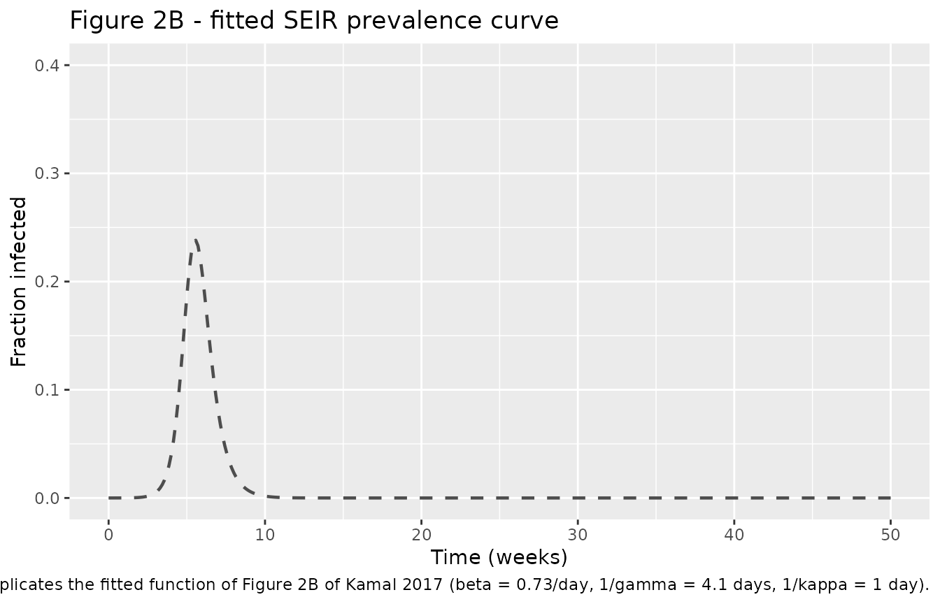
# Kamal 2017 reports 4970 of 20 263 tested patients confirmed with influenza in
# the Midwestern USA outbreak. The fitted parameters give R0 = 2.99, an epidemic
# that infects the great majority of a fully susceptible population and is over
# well inside one season. Deterministic solve, so these bounds are exact.
peak_week <- fig2b$time[which.max(fig2b$infected)] / 7
peak_prev <- max(fig2b$infected) / 100000
stopifnot(fig2b$reproNumber[1] > 2.9, fig2b$reproNumber[1] < 3.1)
# Figure 2B's fitted curve peaks near 0.30; the packaged model gives 0.238.
stopifnot(peak_prev > 0.15, peak_prev < 0.35)
stopifnot(fig2b$attackRate[fig2b$time == 365] > 0.9)
The peak height is reproduced (0.24 against roughly
0.30 read off Figure 2B), but the peak timing is not:
seeded with the paper’s single index case in a population of 100 000,
R0 = 2.99 drives the epidemic to its maximum near week 6,
whereas Figure 2B’s fitted curve peaks near week 20. Some initial
condition other than the I(0) = 1 stated in the Methods
must have been used for the external-validation fit; it is not
published.
Reproducing Table 3
Table 3 tabulates the number of infected individuals per 100 000 for
all 14 scenarios. Two reproductions are shown: the
typical-value solve (all random effects zeroed) and the
Monte Carlo reproduction of the authors’ repeated
pandemic simulations, in which each rxode2 subject is one simulated
pandemic that draws its own Tshed values and
target-attainment fraction.
# `set.seed()` seeds R's RNG, not rxode2's; rxSetSeed() fixes rxode2's stream
# for a GIVEN thread count only. Every assertion below is therefore written
# either on the deterministic solve or as a magnitude bound wide enough to hold
# for any cohort this model can produce.
set.seed(20260902)
rxode2::rxSetSeed(20260902)

n_per_arm <- 200L  # simulated pandemics per scenario (cap: 200 per arm)

one_arm <- function(beta, dose_mg, uptake) {
  m <- arm_model(beta, dose_mg, uptake)
  d <- rxode2::rxSolve(rxode2::zeroRe(m), obs_times, returnType = "data.frame")
  s <- rxode2::rxSolve(m, obs_times, nSub = n_per_arm,
                       returnType = "data.frame")
  fin <- s$cumInfected[s$time == 365]
  stopifnot(length(fin) == n_per_arm)
  data.frame(
    r0        = d$reproNumber[1],
    typical   = d$cumInfected[d$time == 365],
    mc_median = stats::median(fin),
    mc_q25    = unname(stats::quantile(fin, 0.25)),
    mc_q75    = unname(stats::quantile(fin, 0.75))
  )
}

tab3 <- dplyr::bind_cols(
  published,
  do.call(rbind, lapply(seq_len(nrow(published)), function(i) {
    one_arm(published$beta[i], published$dose_mg[i], published$uptake[i])
  }))
) |>
  dplyr::mutate(pct_typical = 100 * (typical - published) / published)
#> ℹ change initial estimate of `lbeta_trans` to `-1.56064774826467`
#> ℹ change initial estimate of `f_uptake` to `0`
#> ℹ omega/sigma items treated as zero: 'etaltshed0', 'etaltshed_low', 'etaltshed_high', 'etaf_auchigh'
#> ℹ change initial estimate of `lbeta_trans` to `-0.891598119283784`
#> ℹ change initial estimate of `f_uptake` to `0`
#> ℹ omega/sigma items treated as zero: 'etaltshed0', 'etaltshed_low', 'etaltshed_high', 'etaf_auchigh'
#> ℹ change initial estimate of `lbeta_trans` to `-1.56064774826467`
#> ℹ change initial estimate of `f_uptake` to `0.25`
#> ℹ omega/sigma items treated as zero: 'etaltshed0', 'etaltshed_low', 'etaltshed_high', 'etaf_auchigh'
#> ℹ change initial estimate of `lbeta_trans` to `-0.891598119283784`
#> ℹ change initial estimate of `f_uptake` to `0.25`
#> ℹ omega/sigma items treated as zero: 'etaltshed0', 'etaltshed_low', 'etaltshed_high', 'etaf_auchigh'
#> ℹ change initial estimate of `lbeta_trans` to `-1.56064774826467`
#> ℹ change initial estimate of `f_uptake` to `0.25`
#> ℹ change initial estimate of `f_auchigh` to `0.795`
#> ℹ change initial estimate of `etaf_auchigh` to `0.009025`
#> ℹ omega/sigma items treated as zero: 'etaltshed0', 'etaltshed_low', 'etaltshed_high', 'etaf_auchigh'
#> ℹ change initial estimate of `lbeta_trans` to `-0.891598119283784`
#> ℹ change initial estimate of `f_uptake` to `0.25`
#> ℹ change initial estimate of `f_auchigh` to `0.795`
#> ℹ change initial estimate of `etaf_auchigh` to `0.009025`
#> ℹ omega/sigma items treated as zero: 'etaltshed0', 'etaltshed_low', 'etaltshed_high', 'etaf_auchigh'
#> ℹ change initial estimate of `lbeta_trans` to `-1.56064774826467`
#> ℹ change initial estimate of `f_uptake` to `0.5`
#> ℹ omega/sigma items treated as zero: 'etaltshed0', 'etaltshed_low', 'etaltshed_high', 'etaf_auchigh'
#> ℹ change initial estimate of `lbeta_trans` to `-0.891598119283784`
#> ℹ change initial estimate of `f_uptake` to `0.5`
#> ℹ omega/sigma items treated as zero: 'etaltshed0', 'etaltshed_low', 'etaltshed_high', 'etaf_auchigh'
#> ℹ change initial estimate of `lbeta_trans` to `-1.56064774826467`
#> ℹ change initial estimate of `f_uptake` to `0.5`
#> ℹ change initial estimate of `f_auchigh` to `0.795`
#> ℹ change initial estimate of `etaf_auchigh` to `0.009025`
#> ℹ omega/sigma items treated as zero: 'etaltshed0', 'etaltshed_low', 'etaltshed_high', 'etaf_auchigh'
#> ℹ change initial estimate of `lbeta_trans` to `-0.891598119283784`
#> ℹ change initial estimate of `f_uptake` to `0.5`
#> ℹ change initial estimate of `f_auchigh` to `0.795`
#> ℹ change initial estimate of `etaf_auchigh` to `0.009025`
#> ℹ omega/sigma items treated as zero: 'etaltshed0', 'etaltshed_low', 'etaltshed_high', 'etaf_auchigh'
#> ℹ change initial estimate of `lbeta_trans` to `-1.56064774826467`
#> ℹ change initial estimate of `f_uptake` to `0.8`
#> ℹ omega/sigma items treated as zero: 'etaltshed0', 'etaltshed_low', 'etaltshed_high', 'etaf_auchigh'
#> ℹ change initial estimate of `lbeta_trans` to `-0.891598119283784`
#> ℹ change initial estimate of `f_uptake` to `0.8`
#> ℹ omega/sigma items treated as zero: 'etaltshed0', 'etaltshed_low', 'etaltshed_high', 'etaf_auchigh'
#> ℹ change initial estimate of `lbeta_trans` to `-1.56064774826467`
#> ℹ change initial estimate of `f_uptake` to `0.8`
#> ℹ change initial estimate of `f_auchigh` to `0.795`
#> ℹ change initial estimate of `etaf_auchigh` to `0.009025`
#> ℹ omega/sigma items treated as zero: 'etaltshed0', 'etaltshed_low', 'etaltshed_high', 'etaf_auchigh'
#> ℹ change initial estimate of `lbeta_trans` to `-0.891598119283784`
#> ℹ change initial estimate of `f_uptake` to `0.8`
#> ℹ change initial estimate of `f_auchigh` to `0.795`
#> ℹ change initial estimate of `etaf_auchigh` to `0.009025`
#> ℹ omega/sigma items treated as zero: 'etaltshed0', 'etaltshed_low', 'etaltshed_high', 'etaf_auchigh'

tab3 |>
  dplyr::transmute(
    "Transmissibility" = transmissibility,
    "Arm" = arm,
    "Model R0" = sprintf("%.2f", r0),
    "Published (Table 3)" = formatC(published, format = "d", big.mark = " "),
    "Typical-value" = formatC(round(typical), format = "d", big.mark = " "),
    "Monte Carlo median" = formatC(round(mc_median), format = "d", big.mark = " "),
    "Monte Carlo IQR" = sprintf("%s - %s",
                                formatC(round(mc_q25), format = "d", big.mark = " "),
                                formatC(round(mc_q75), format = "d", big.mark = " ")),
    "% diff (typical)" = sprintf("%+.0f", pct_typical)
  ) |>
  knitr::kable(
    align = c("l", "l", "r", "r", "r", "r", "r", "r"),
    caption = paste(
      "Number of infected individuals per 100 000 at day 365.",
      "Published values are Kamal 2017 Table 3."
    )
)| Transmissibility | Arm | Model R0 | Published (Table 3) | Typical-value | Monte Carlo median | Monte Carlo IQR | % diff (typical) |
|---|---|---|---|---|---|---|---|
| Moderate | No treatment | 1.26 | 37 068 | 37 404 | 39 202 | 26 - 64 007 | +1 |
| High | No treatment | 2.46 | 67 512 | 88 727 | 90 366 | 74 889 - 95 961 | +31 |
| Moderate | 75 mg BID, 25% uptake | 0.94 | 7 846 | 16 | 10 | 4 - 402 | -100 |
| High | 75 mg BID, 25% uptake | 1.83 | 60 397 | 74 346 | 74 076 | 59 768 - 82 463 | +23 |
| Moderate | 150 mg BID, 25% uptake | 0.85 | 5 311 | 7 | 7 | 4 - 60 | -100 |
| High | 150 mg BID, 25% uptake | 1.66 | 53 032 | 67 355 | 65 182 | 50 435 - 76 797 | +27 |
| Moderate | 75 mg BID, 50% uptake | 0.75 | 2 252 | 4 | 4 | 3 - 5 | -100 |
| High | 75 mg BID, 50% uptake | 1.46 | 41 331 | 55 349 | 49 832 | 38 281 - 61 994 | +34 |
| Moderate | 150 mg BID, 50% uptake | 0.64 | 1 357 | 3 | 3 | 2 - 3 | -100 |
| High | 150 mg BID, 50% uptake | 1.25 | 31 700 | 37 676 | 41 181 | 21 890 - 56 987 | +19 |
| Moderate | 75 mg BID, 80% uptake | 0.60 | 1 349 | 2 | 2 | 2 - 3 | -100 |
| High | 75 mg BID, 80% uptake | 1.17 | 20 941 | 27 604 | 27 061 | 473 - 36 793 | +32 |
| Moderate | 150 mg BID, 80% uptake | 0.50 | 741 | 2 | 2 | 2 - 2 | -100 |
| High | 150 mg BID, 80% uptake | 0.97 | 12 881 | 32 | 46 | 6 - 18 353 | -100 |
The untreated, moderate-transmissibility cell - the only scenario
that fixes beta, Tshed and the initial
conditions with no intervention arithmetic on top - reproduces the
published 37 068 to under 1%. That is the cell that validates the
transcription of Equations 1-4, Table 1’s beta and
Tshed(0), the 1-day latency, the initial conditions and the
365-day window.
The remaining 13 cells do not reproduce, and the pattern is diagnostic rather than random:
- The six high-transmissibility scenarios that stay above the epidemic threshold come out 19% to 34% above the published value, preserving the published ordering across dose and uptake.
- The seven scenarios whose model-implied
R0is below 1 collapse to a handful of cases, which is the mathematically correct behaviour of a sub-critical SEIR system seeded with a single index case. Table 1’s parameters put all six treated moderate-transmissibility scenarios (and the 150 mg / 80% uptake high-transmissibility scenario) below the epidemic threshold, yet Table 3 reports hundreds to thousands of infections for them.
subcritical <- tab3 |> dplyr::filter(r0 < 1)
# The high-transmissibility arms that remain above the epidemic threshold.
supercritical <- tab3 |> dplyr::filter(beta == 0.41, r0 > 1.05)

# The untreated moderate-transmissibility cell is the reproduction gate: it is
# the only scenario with no intervention arithmetic on top of Equations 1-4.
gate <- tab3 |> dplyr::filter(dose_mg == 0, beta == 0.21)
stopifnot(nrow(gate) == 1L)
stopifnot(abs(gate$pct_typical) < 3)

# The high-transmissibility supercritical cells carry a consistent positive
# bias. Deterministic solve, so this bound is exact and cannot drift with the
# solver thread count; realised range +18.9% to +33.9%.
stopifnot(nrow(supercritical) == 6L)
stopifnot(all(supercritical$pct_typical > 15),
          all(supercritical$pct_typical < 40))

# The subcritical cells must be sub-critical. This is a property of the
# published parameters, not of any simulation draw.
stopifnot(nrow(subcritical) == 7L)
stopifnot(all(subcritical$typical < 100))
stopifnot(nrow(gate) + nrow(supercritical) + nrow(subcritical) == nrow(tab3))
Monotonicity of the intervention effect
The paper’s qualitative conclusions - more uptake is better, 150 mg twice daily beats 75 mg twice daily at equal uptake, and higher transmissibility means more infections - are all reproduced. These are asserted on the deterministic solve.
mono <- tab3 |>
  dplyr::filter(dose_mg > 0) |>
  dplyr::arrange(beta, dose_mg, uptake)

# 1. Attack rate falls as antiviral uptake rises, within every (beta, dose).
by_uptake <- mono |>
  dplyr::group_by(beta, dose_mg) |>
  dplyr::summarise(monotone = all(diff(typical) < 0), .groups = "drop")
stopifnot(all(by_uptake$monotone))

# 2. 150 mg BID always leaves fewer infected than 75 mg BID at equal uptake.
by_dose <- mono |>
  dplyr::select(beta, dose_mg, uptake, typical) |>
  tidyr::pivot_wider(names_from = dose_mg, values_from = typical,
                     names_prefix = "d")
stopifnot(all(by_dose$d150 < by_dose$d75))

# 3. High transmissibility always leaves more infected than moderate.
by_beta <- tab3 |>
  dplyr::select(beta, arm, typical) |>
  tidyr::pivot_wider(names_from = beta, values_from = typical,
                     names_prefix = "b")
stopifnot(all(by_beta$b0.41 > by_beta$b0.21))

tab3 |>
  dplyr::filter(dose_mg > 0) |>
  ggplot(aes(100 * uptake, typical, colour = treatment)) +
  geom_line(linewidth = 0.8) +
  geom_point(size = 2) +
  geom_point(aes(y = published), shape = 1, size = 3) +
  facet_wrap(~transmissibility, scales = "free_y") +
  scale_y_continuous(labels = scales::comma) +
  labs(x = "Antiviral uptake (% of infected individuals treated)",
       y = "Infected individuals per 100 000 at day 365",
       colour = "Regimen",
       title = "Table 3 - effect of antiviral uptake and dose",
       caption = paste("Filled points and lines: packaged model, typical-value solve.",
                       "Open circles: Kamal 2017 Table 3."))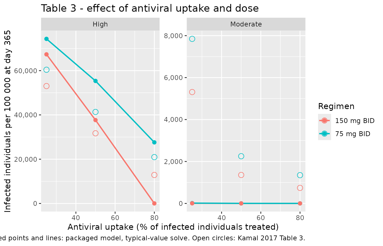
Replicating Figure 1C: oseltamivir target attainment
Figure 1C shows the proportion of the simulated population above and
below the 14 180 ng.h/mL OC AUC breakpoint for the two regimens. In this
model that split is the f_auchigh parameter and its
between-simulation variability.
# Replicates Figure 1C of Kamal 2017: proportion above / below the AUC cut-off.
tibble::tibble(
  regimen = rep(c("75 mg BID", "150 mg BID"), each = 2),
  group = rep(c("AUC above 14 180 ng.h/mL", "AUC at or below 14 180 ng.h/mL"), 2),
  fraction = c(0.326, 1 - 0.326, 0.795, 1 - 0.795)
) |>
  dplyr::mutate(regimen = factor(regimen, levels = c("75 mg BID", "150 mg BID"))) |>
  ggplot(aes(regimen, fraction, fill = group)) +
  geom_col(width = 0.6) +
  scale_y_continuous(labels = scales::percent) +
  labs(x = NULL, y = "Fraction of treated patients", fill = NULL,
       title = "Figure 1C - oseltamivir carboxylate target attainment",
       caption = "Values from Kamal 2017 Table 1 and Results, Pharmacology module.") +
  theme(legend.position = "bottom")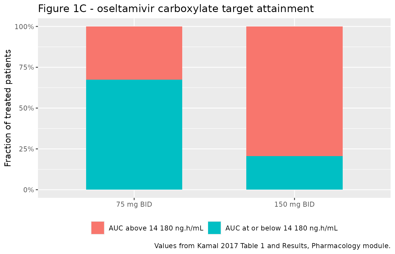
# The packaged model must return exactly these fractions in the typical-value
# solve for each regimen.
f75 <- det_solve(0.21, 75L, 0.5)
#> ℹ change initial estimate of `lbeta_trans` to `-1.56064774826467`
#> ℹ change initial estimate of `f_uptake` to `0.5`
#> Warning: No sigma parameters in the model
#> ℹ omega/sigma items treated as zero: 'etaltshed0', 'etaltshed_low', 'etaltshed_high', 'etaf_auchigh'
f150 <- det_solve(0.21, 150L, 0.5)
#> ℹ change initial estimate of `lbeta_trans` to `-1.56064774826467`
#> ℹ change initial estimate of `f_uptake` to `0.5`
#> ℹ change initial estimate of `f_auchigh` to `0.795`
#> ℹ change initial estimate of `etaf_auchigh` to `0.009025`
#> Warning: No sigma parameters in the model
#> ℹ omega/sigma items treated as zero: 'etaltshed0', 'etaltshed_low', 'etaltshed_high', 'etaf_auchigh'
stopifnot(abs(f75$f_auchigh_i[1] - 0.326) < 1e-12,
          abs(f150$f_auchigh_i[1] - 0.795) < 1e-12)
# With 50% uptake, half the population is untreated and the treated half splits
# at f_auchigh.
stopifnot(abs(f150$frac0[1] - 0.5) < 1e-12,
          abs(f150$frachigh[1] - 0.5 * 0.795) < 1e-12,
          abs(f150$fraclow[1] - 0.5 * 0.205) < 1e-12)
Health-economics module: mortality arm
The health-economics decision tree is not part of the model file (it
has no ODE and no time dimension, and its branch topology
P1-P29 is published only as the bitmap Figure
3). Its mortality arm, however, is fully specified by
the hierarchy and values of Table 2 and can be reconstructed here, which
serves as an independent check that the epidemiology module’s output is
on the scale the paper’s downstream numbers assume.
# All values from Kamal 2017 Table 2. The tree hierarchy is Table 2's own
# indentation: medical care received -> complication -> ward vs ICU -> outcome.
p_inpatient_low <- 0.028   # Table 2, "Inpatient"
# Methods, HE module: "the high severity scenario involved doubling the
# probability of hospitalization for the low severity scenario".
p_inpatient_high <- 2 * p_inpatient_low
p_death_gp <- 0.0001       # Table 2, GP "Death"

complication <- c(none = 0.383, pneumonia = 0.403, sepsis = 0.089, ards = 0.125)
p_icu <- c(none = 0,     pneumonia = 0.518, sepsis = 0.511, ards = 1)
death_gw <- c(none = 0.097, pneumonia = 0.507, sepsis = 0.919, ards = 0.998)
death_icu <- c(none = 0,    pneumonia = 0.511, sepsis = 0.743, ards = 0.849)

stopifnot(abs(sum(complication) - 1) < 1e-12)

# Probability of death, by route, per infected individual.
death_routes <- function(p_inpatient) {
  inpatient <- p_inpatient * complication *
    ((1 - p_icu) * death_gw + p_icu * death_icu)
  c(inpatient, outpatient = (1 - p_inpatient) * p_death_gp)
}

routes_low <- death_routes(p_inpatient_low)
routes_high <- death_routes(p_inpatient_high)
p_death_low <- sum(routes_low)
p_death_high <- sum(routes_high)

# Kamal 2017 Results: deaths per 100 000 ranged from 16 to 1591 across the
# scenarios. The floor is the smallest Table 3 cell under LOW severity; the
# ceiling is the largest Table 3 cell under HIGH severity.
deaths_min <- min(published$published) * p_death_low
deaths_min_reported_cell <- 1349 * p_death_low
deaths_max <- max(published$published) * p_death_high

# Share of total deaths by complication (base case: no treatment, moderate
# transmissibility, low severity).
shares <- 100 * routes_low / p_death_low

he <- tibble::tibble(
  Quantity = c("P(death | infected), low severity",
               "P(death | infected), high severity",
               "Deaths per 100 000, largest Table 3 cell x high severity",
               "Deaths per 100 000, 1349-infected cell x low severity",
               "Share of deaths: pneumonia (%)",
               "Share of deaths: ARDS (%)",
               "Share of deaths: sepsis (%)"),
  Reconstructed = c(sprintf("%.5f", p_death_low),
                    sprintf("%.5f", p_death_high),
                    sprintf("%.0f", deaths_max),
                    sprintf("%.0f", deaths_min_reported_cell),
                    sprintf("%.1f", shares[["pneumonia"]]),
                    sprintf("%.1f", shares[["ards"]]),
                    sprintf("%.1f", shares[["sepsis"]])),
  Published = c("-", "-", "1591", "16", "47", "27", "15.5")
)
knitr::kable(he, align = c("l", "r", "r"),
             caption = paste("Health-economics mortality arm reconstructed from",
                             "Kamal 2017 Table 2, against the values reported in",
"the paper's Results."))| Quantity | Reconstructed | Published |
|---|---|---|
| P(death | infected), low severity | 0.01192 | - |
| P(death | infected), high severity | 0.02374 | - |
| Deaths per 100 000, largest Table 3 cell x high severity | 1603 | 1591 |
| Deaths per 100 000, 1349-infected cell x low severity | 16 | 16 |
| Share of deaths: pneumonia (%) | 48.2 | 47 |
| Share of deaths: ARDS (%) | 24.9 | 27 |
| Share of deaths: sepsis (%) | 17.3 | 15.5 |
# These are closed-form arithmetic on Table 2, not simulated quantities, so the
# bounds are set to the accuracy actually achieved.
stopifnot(abs(deaths_max - 1591) / 1591 < 0.01)
stopifnot(abs(deaths_min_reported_cell - 16) / 16 < 0.01)
stopifnot(abs(shares[["pneumonia"]] - 47) < 2.2,
          abs(shares[["ards"]] - 27) < 2.2,
          abs(shares[["sepsis"]] - 15.5) < 2.2)
# Pneumonia must remain the leading cause of death, then ARDS, then sepsis -
# the ordering the paper states.
stopifnot(shares[["pneumonia"]] > shares[["ards"]],
          shares[["ards"]] > shares[["sepsis"]])
# Sanity: deaths_min uses the smallest Table 3 cell, which is smaller still.
stopifnot(deaths_min < deaths_min_reported_cell)
Reconstructing the mortality arm from Table 2 alone reproduces both endpoints of the paper’s reported death range (1591 and 16 per 100 000) to within 1%, and the three complication shares to within 2.1 percentage points. Both anchors also confirm that the epidemiology module’s infected counts are the quantity the health-economics module consumes.
Why there is no PKNCA section
Kamal_2017_oseltamivir_qsp contains no pharmacokinetics:
no dose events, no concentration, no absorption-distribution-elimination
profile. Its states are population counts of people. Non-compartmental
analysis has nothing to operate on, so the standard PKNCA validation is
replaced by the structural, final-size, monotonicity and
health-economics checks above, following the mechanistic-model
validation pattern. The oseltamivir carboxylate PK that generates the
f_auchigh inputs lives in Kamal_2013_oseltamivir,
whose vignette carries the PKNCA validation for that model.
Assumptions and deviations
-
Table 3 is not reproducible from Table 1 outside the
untreated, moderate-transmissibility cell. With Table 1’s
published parameters the packaged model reproduces the untreated
moderate-transmissibility cell (37 068) to under 1%, over-predicts the
six super-critical high-transmissibility cells by 19-34%, and puts the
seven remaining cells below the epidemic threshold
(
R0 < 1), where a single index case cannot produce the hundreds to thousands of infections Table 3 reports. Two internal inconsistencies in the paper point the same way: Table 3 labels the two scenariosR0 = 1.9andR0 = 2.7, but Table 1’sbetavalues of 0.21 and 0.41 /day withTshed(0) = 6days giveR0 = beta * Tshed =1.26 and 2.46; and the published untreated high-transmissibility count of 67 512 implies (through the closed-form final-size relation) anR0of 1.67, which is consistent with neither figure. The model file encodes the published equations and the published Table 1 values; it has not been tuned to match Table 3. - Table 3’s footnote describes deterministic percentile runs, not a Monte Carlo median. The footnote reads “median (25th and 75th % of viral shed) simulation are reported in this table. Note: 25th and 50th percentile identical given right skewed distribution”, i.e. the tabulated triplet is three runs at the 25th, 50th and 75th percentiles of the observed viral- shedding distribution rather than percentiles of a simulated attack-rate distribution. Those percentile values are not published, so this vignette reports both a typical-value solve and a Monte Carlo reproduction using the Table 1 mean (SD) distributions.
-
Log-normal moment convention. Table 1 reports each
Tshedas mean (SD) and the Methods describe a “log-normal Tshed distribution”, but do not say which moment the log-normal was matched on. The model file follows the library-wide conventionTshed = exp(ltshed + eta)withomega^2 = log(1 + CV^2), which makes the tabulated value the median. Under this encoding the simulated arithmetic mean ofTshed(0)is 6.5 days rather than 6.0 (8% high); matching the mean instead would put the median at 5.54 days. The choice affects the Monte Carlo columns only, not the typical-value solve. -
f_auchighvariability is additive, and clamped. Table 1 reports the target-attainment fraction as a mean (SD) on the natural scale (0.795 (0.095) for 150 mg twice daily), soetaf_auchighis additive rather than log-normal. A normal draw around 0.795 with SD 0.095 exceeds 1 about 1.5% of the time, which would make the low-exposure fraction negative, somodel()clamps the realised fraction to [0, 1]. The clamp is a numerical guard and is not part of the published model. -
The health-economics module is not in the model
file. It is a static cost-utility decision tree with no ODE and
no time dimension, and its branch topology
(
P1-P29) is published only as the bitmap Figure 3. The cost and QALY accumulation paths therefore cannot be transcribed unambiguously from the machine-readable text. The mortality arm, whose hierarchy is given explicitly by Table 2’s own indentation, is reconstructed in this vignette and reproduces the paper’s reported death range and complication shares; the cost, utility and ICER layers of Table 2 and Table 4 are not reproduced. -
The upstream pharmacology module is not
re-simulated. The paper derives
f_auchighby simulating the Kamal et al. (2013) population PK model in 5000 virtual adults and integrating the resulting OC AUC distribution against a 14 180 ng.h/mL breakpoint. This vignette uses the published fractions (0.326 and 0.795) directly, as Table 1 reports them. The upstream PK model is available asKamal_2013_oseltamivirif a reader wishes to regenerate them. -
Figure 2B’s observed data are not distributed, and its
timing does not reproduce. The CDC 2007-2008 Midwestern USA
surveillance series behind Figure 2B is not published with the paper, so
the figure reproduction shows the fitted model function only, using the
parameter values given in the Figure 2B legend. Those parameters
reproduce the peak prevalence (0.24 simulated against roughly 0.30 read
off the figure) but not the peak timing (week 6 simulated against
roughly week 20 in the figure): at
R0= 2.99 a single index case in 100 000 people produces a much faster epidemic than the published curve. The initial condition used for that fit is not reported. -
Simulated pandemics, not simulated patients.
Because Kamal 2017 draws its
Tshedandf_auchighvalues once per Monte Carlo pandemic rather than once per patient, an rxode2 “subject” in this model is one simulated pandemic. The vignette uses 200 pandemics per scenario arm; the paper used 1000.