Acalabrutinib and ACP-5862 in Chinese and White patients (Yao 2025)
Source:vignettes/articles/Yao_2025_acalabrutinib.Rmd
Yao_2025_acalabrutinib.RmdModel and source
- Citation: Yao T, Ding J, Sharma S, Li Y, Xu Q, Ma P. Assessment of ethnic differences in pharmacokinetics and clinical responses of acalabrutinib between Chinese and White patients with B-cell malignancies. Br J Clin Pharmacol. 2025;91(7):2008-2019. doi:10.1002/bcp.70018
- Article: https://doi.org/10.1002/bcp.70018 (open access)
Yao 2025 adds a Chinese phase 1/2 study (NCT03932331, n = 105) and a
Japanese phase 1 study (NCT03198650, n = 6) to the global acalabrutinib
/ ACP-5862 population PK dataset and re-estimates the existing Edlund
2022 model (modellib("Edlund_2022_acalabrutinib")) with one
addition: an East Asian race effect on the relative bioavailability F1
(+22.6%) and on the peripheral volume of acalabrutinib (-38.1%). It then
relates the model-predicted steady-state exposures to efficacy (Chinese
patients only; graphical) and to safety (476 patients; logistic
regression). The paper contributes three models:
| Model | Content |
|---|---|
Yao_2025_acalabrutinib |
Joint acalabrutinib / ACP-5862 population PK model (Table 3) |
Yao_2025_acalabrutinib_teae_grade2 |
Logistic regression of any grade >= 2 adverse event on acalabrutinib AUC24h,ss (Figure 6, left) |
Yao_2025_acalabrutinib_teae_grade3 |
Logistic regression of any grade >= 3 adverse event on acalabrutinib AUC24h,ss (Figure 6, right) |
The PK model is a joint parent-metabolite model: acalabrutinib is
absorbed through a dosing depot, five transit compartments and an
absorption depot, distributes into two compartments, and is cleared at
CL/F, of which the fraction fm = 0.4 forms ACP-5862, which
itself has two-compartment disposition (Figure 1).
Population
The PK dataset held 11152 acalabrutinib and 3367 ACP-5862 concentrations from 14 clinical trials: 138 healthy subjects and 686 patients with B-cell malignancies. By race (Figure 3 caption) there were 622 White, 105 Chinese, 6 Japanese, 47 Black or African American and 44 other subjects. The paper reports demographics only for the Chinese cohort (Tables 1 and 2): 75 men and 30 women, mean age 60.5 years, mean weight 65.9 kg, mean creatinine clearance 74.7 mL/min; CLL 64, MCL 34, FL 4, SLL 2 and DLBCL 1; ECOG 0 / 1 / 2 in 66 / 35 / 4 patients; one PPI user.
The exposure-safety analysis pooled 476 patients from six global studies and the China study (Supplementary Table S1): 440 received 100 mg BID, and the others 100-250 mg QD or 200 mg BID.
The same information is available programmatically via
readModelDb("Yao_2025_acalabrutinib")()$population.
Source trace
Every ini() value carries an in-file comment pointing at
its source. The table collects them.
| Equation / parameter | Value | Source location |
|---|---|---|
lcl (CL/F) |
log(130.3) L/h | Table 3 |
lvc (Vc/F) |
log(28.8) L | Table 3 |
lq (Q/F) |
log(19.5) L/h | Table 3 |
lvp (Vp/F) |
log(105.6) L | Table 3 |
lka (Ka) |
log(1.4) 1/h | Table 3 |
lmtt (MTT) |
log(0.4) h | Table 3 |
ntr |
5 (not estimated) | Methods “Pop-PK analysis”; Figure 1 |
lfdepot (F1) |
log(1) (reference) | No F1 row in Table 3; F1 carries BOV and covariates only |
fm |
0.4 (not estimated) | Methods “Pop-PK analysis” |
lcl_acp (CLM/F) |
log(21.5) L/h | Table 3 |
lvc_acp (VcM/F) |
log(24.3) L | Table 3 |
lq_acp (QM/F) |
log(21.1) L/h | Table 3 |
lvp_acp (VpM/F) |
log(90.9) L | Table 3 |
e_dis_healthy_cl, e_dis_healthy_vp
|
0.645, -0.424 | Table 3 (HEALTHGP rows); Results “Covariates analysis result” |
e_ecog_ge2_cl |
-0.128 | Table 3 (CL/F_ECOG2+) |
e_conmed_ppi_fdepot |
-0.307 | Table 3 (F1_PPI) |
e_race_asian_northeast_vp,
e_race_asian_northeast_fdepot
|
-0.381, 0.226 | Table 3 (EASTASIA rows); Results “Effect of race covariate” |
etalcl, etalvc, etalvp
|
0.0524, 2.34, 0.121 | Table 3 BSV 23.2, 306, 35.9 (CV%) |
etalcl_acp, etalvc_acp,
etalq_acp, etalvp_acp
|
0.0173, 0.131, 0.329, 0.0824 | Table 3 BSV 13.2, 37.4, 62.4, 29.3 (CV%) |
etaiov_mtt_1..4 |
0.941 | Table 3 BOV MTT 125 (CV%); four occasions (footnote a) |
etaiov_fdepot_1..4 |
0.247 | Table 3 BOV F1 52.9 (CV%) |
expSdIntensive, expSdSparse
|
0.641, 0.925 | Table 3 RE parent, rich and sparse (SD) |
expSdIntensive_acp, expSdSparse_acp
|
0.36, 0.401 | Table 3 RE metabolite, rich and sparse (SD) |
Covariate form TVP * (1 + Pcov)
|
n/a | Methods equation; Table 3 footnote b |
Transit chain, absorption depot,
ktr = (ntr + 1) / mtt
|
n/a | Figure 1 and its legend |
Molar formation fm * CL/F * Cp into ACP-5862 |
n/a | Methods; MW acalabrutinib 465.5 (Methods “E-R analyses”) |
| Log-scale residual error, rich vs sparse | n/a | Methods “Pop-PK analysis” |
logit_ref, e_auc_logit (grade >=
2) |
1.851, 0.0003197 per ng*h/mL | Figure 6 left panel, digitised fitted line (P = 0.12) |
logit_ref, e_auc_logit (grade >=
3) |
0.0157, 0.0001807 per ng*h/mL | Figure 6 right panel, digitised fitted line (P = 0.051) |
Simulation design
The exposures of Figure 3 are steady-state AUC24h,ss and Cmax,ss at
100 mg BID. Two cohorts of 200 patients (ECOG 0-1, no PPI) are
simulated: a non-East Asian reference and an East Asian cohort that
differs only in RACE_ASIAN_NORTHEAST. The same random
effects are used in both cohorts (common random numbers), so the cohort
difference is the race effect alone.
Following the procedure of the Edlund 2022 analysis that this model
extends, each dose draws its own F1 and MTT from the
between-occasion distributions: every record stays on
OCC = 1 and etaiov_mtt_1 /
etaiov_fdepot_1 are supplied as event-table columns that
change at every dose. All random effects are drawn in R and passed with
omega = NA, so the cohort is identical on every machine.
AUC24h,ss is the AUC over a 7-day steady-state window divided by 7, and
Cmax,ss the mean of the 14 per-dose maxima.
mod <- readModelDb("Yao_2025_acalabrutinib")
ui <- rxode2::rxode2(mod)
#> ℹ parameter labels from comments will be replaced by 'label()'
#> Warning: some etas defaulted to non-mu referenced, possible parsing error: etaiov_mtt_1, etaiov_mtt_2, etaiov_mtt_3, etaiov_mtt_4, etaiov_fdepot_1, etaiov_fdepot_2, etaiov_fdepot_3, etaiov_fdepot_4
#> as a work-around try putting the mu-referenced expression on a simple line
om <- ui$omega

n_sub <- 200
tau <- 12
n_run_in <- 6 # three days of BID dosing to reach steady state
n_window <- 14 # a 7-day steady-state window
t_win <- c(n_run_in * tau, (n_run_in + n_window) * tau)
dose_times <- (seq_len(n_run_in + n_window + 1) - 1) * tau

set.seed(20250226)
# Between-subject etas: Latin-hypercube quantiles so every marginal is
# reproduced exactly at n = 200 while the etas stay mutually independent.
lhs <- function(v) sqrt(v) * qnorm((sample.int(n_sub) - 0.5) / n_sub)
bsv_names <- c("etalcl", "etalvc", "etalvp", "etalcl_acp", "etalvc_acp",
               "etalq_acp", "etalvp_acp")
subj <- tibble(id = seq_len(n_sub))
for (nm in bsv_names) subj[[nm]] <- lhs(om[nm, nm])

# One BOV draw per dose and subject.
dose_iov <- expand.grid(dose_k = seq_along(dose_times), id = seq_len(n_sub)) |>
  as_tibble() |>
  mutate(
    time = dose_times[dose_k],
    etaiov_mtt_1 = rnorm(n(), 0, sqrt(om["etaiov_mtt_1", "etaiov_mtt_1"])),
    etaiov_fdepot_1 = rnorm(n(), 0, sqrt(om["etaiov_fdepot_1", "etaiov_fdepot_1"]))
  )

# Dense (0.1 h) over the first 4 h after each dose, where the peak lies,
# 0.5 h over the rest of the interval.
tad_grid <- c(seq(0, 4, by = 0.1), seq(4.5, tau - 0.5, by = 0.5))
obs_times <- c(as.vector(outer(tad_grid, seq(t_win[1], t_win[2] - tau, by = tau), "+")),
               t_win[2])

make_arm <- function(arm, east_asian, id_offset) {
  doses <- dose_iov |>
    mutate(evid = 1L, amt = 100, cmt = "depot", dvid = NA_integer_)
  obs <- expand.grid(time = obs_times, id = seq_len(n_sub)) |>
    as_tibble() |>
    mutate(evid = 0L, amt = 0, cmt = "central", dvid = 1L)
  bind_rows(doses, obs) |>
    arrange(id, time, desc(evid)) |>
    group_by(id) |>
    tidyr::fill(dose_k, etaiov_mtt_1, etaiov_fdepot_1) |>
    ungroup() |>
    left_join(subj, by = "id") |>
    mutate(
      id = id + id_offset, arm = arm, OCC = 1L, SAMPLE_INTENSIVE = 1L,
      DIS_HEALTHY = 0L, ECOG_GE2 = 0L, CONMED_PPI = 0L,
      RACE_ASIAN_NORTHEAST = east_asian
    )
}

arms <- c("Non-East Asian", "East Asian")
events <- bind_rows(
  make_arm(arms[1], 0L, 0L),
  make_arm(arms[2], 1L, n_sub)
)
stopifnot(!anyDuplicated(events[, c("id", "time", "evid")]))
sim <- suppressWarnings(rxode2::rxSolve(
  mod, events = events, omega = NA, returnType = "data.frame",
  keep = c("arm", "dose_k"), addDosing = FALSE
))
#> ℹ parameter labels from comments will be replaced by 'label()'
sim <- sim |> mutate(arm = factor(arm, levels = arms))

# Harness check: the per-subject etas supplied on the event rows reach the
# model, and the race effect multiplies F1 by exactly 1.226.
par_i <- sim |>
  group_by(id) |>
  slice(1) |>
  ungroup()
stopifnot(
  max(abs(par_i$cl / (130.3 * exp(par_i$etalcl)) - 1)) < 1e-8,
  max(abs(par_i$vp / (105.6 * exp(par_i$etalvp) *
    (1 - 0.381)^(par_i$arm == "East Asian")) - 1)) < 1e-8
)
f_ratio <- sim |>
  filter(time == t_win[1]) |>
  select(arm, id, fdepot) |>
  mutate(sid = (id - 1L) %% n_sub) |>
  select(-id) |>
  pivot_wider(names_from = arm, values_from = fdepot)
stopifnot(max(abs(f_ratio$`East Asian` / f_ratio$`Non-East Asian` - 1.226)) < 1e-8)
Typical-value profiles
A single 100 mg dose for a typical non-East Asian and a typical East Asian patient, all random effects at zero. The East Asian profile is higher through the higher F1; its smaller peripheral volume makes the acalabrutinib distribution phase shorter.
ev_typ <- bind_rows(
  tibble(time = 0, amt = 100, evid = 1L, cmt = "depot", dvid = NA_integer_),
  tibble(time = seq(0, 24, by = 0.05), amt = 0, evid = 0L, cmt = "central",
         dvid = 1L)
)
ev_typ <- bind_rows(
  ev_typ |> mutate(id = 1L, RACE_ASIAN_NORTHEAST = 0L, group = "Non-East Asian"),
  ev_typ |> mutate(id = 2L, RACE_ASIAN_NORTHEAST = 1L, group = "East Asian")
) |>
  mutate(DIS_HEALTHY = 0L, ECOG_GE2 = 0L, CONMED_PPI = 0L, OCC = 1L,
         SAMPLE_INTENSIVE = 1L)
sim_typ <- suppressWarnings(rxode2::rxSolve(
  mod, events = ev_typ, omega = NA, returnType = "data.frame",
  keep = "group", addDosing = FALSE
))

sim_typ |>
  select(time, group, Acalabrutinib = Cc, `ACP-5862` = Cc_acp) |>
  pivot_longer(c(Acalabrutinib, `ACP-5862`), names_to = "analyte", values_to = "conc") |>
  ggplot(aes(time, conc, colour = group)) +
  geom_line() +
  facet_wrap(~analyte) +
  scale_y_log10(limits = c(0.5, NA)) +
  labs(x = "Time after a single 100 mg dose (h)", y = "Concentration (ng/mL)",
       colour = NULL, caption = "Typical-value prediction, random effects at zero.")
#> Warning in scale_y_log10(limits = c(0.5, NA)): log-10 transformation introduced
#> infinite values.
#> Warning: Removed 143 rows containing missing values or values outside the scale range
#> (`geom_line()`).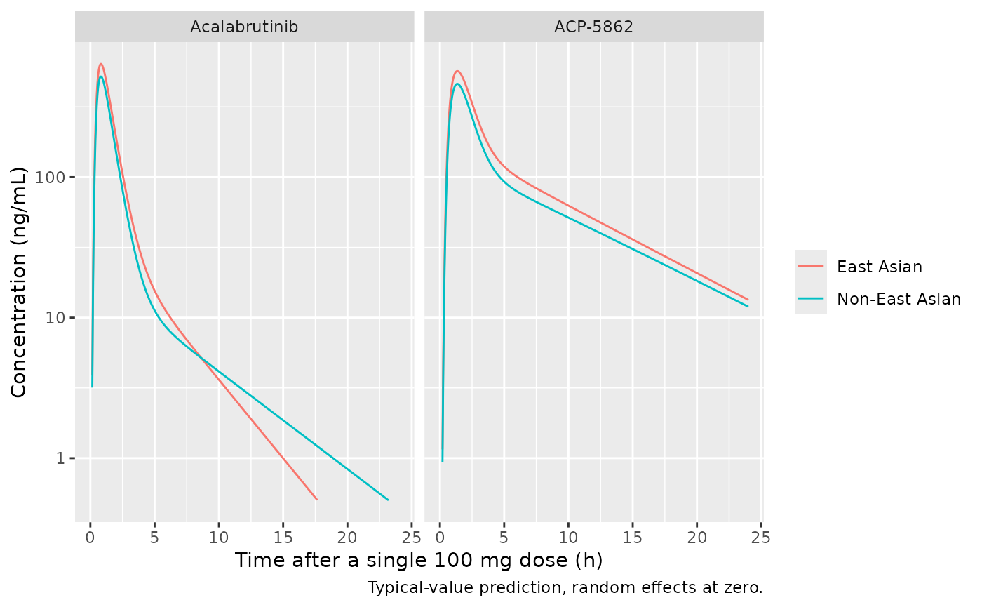
PKNCA validation
PKNCA computes the AUC over the whole 7-day window per subject, analyte and cohort from the simulated profile, sampled every 0.25 h over the first 2 h after each dose and every 0.5 h otherwise. Cmax,ss is the mean of the 14 per-dose maxima on the 0.1 h simulation grid.
conc_long <- sim |>
  filter(!is.na(Cc)) |>
  select(id, time, dose_k, arm, Acalabrutinib = Cc, `ACP-5862` = Cc_acp) |>
  pivot_longer(c(Acalabrutinib, `ACP-5862`), names_to = "analyte", values_to = "Cc") |>
  mutate(treatment = paste(arm, analyte, sep = " | "))

conc_nca <- conc_long |>
  mutate(tad = (time - t_win[1]) %% tau) |>
  filter(abs(time * 2 - round(time * 2)) < 1e-6 |
    (tad < 2 + 1e-6 & abs(time * 4 - round(time * 4)) < 1e-6)) |>
  select(id, time, Cc, treatment)
stopifnot(all(conc_nca |> group_by(id, treatment) |>
  summarise(t0 = min(time), t1 = max(time), .groups = "drop") |>
  with(t0 == t_win[1] & t1 == t_win[2])))

dose_df <- events |>
  filter(evid == 1, time >= t_win[1], time < t_win[2]) |>
  select(id, time, amt, arm) |>
  tidyr::expand_grid(analyte = c("Acalabrutinib", "ACP-5862")) |>
  mutate(treatment = paste(arm, analyte, sep = " | ")) |>
  select(-arm, -analyte)

intervals <- data.frame(start = t_win[1], end = t_win[2], auclast = TRUE)
# One PKNCA call per cohort and analyte keeps each call at 200 subjects.
nca_one <- function(trt) {
  conc_obj <- PKNCA::PKNCAconc(filter(conc_nca, treatment == trt), Cc ~ time | treatment + id)
  dose_obj <- PKNCA::PKNCAdose(filter(dose_df, treatment == trt), amt ~ time | treatment + id)
  res <- PKNCA::pk.nca(PKNCA::PKNCAdata(conc_obj, dose_obj, intervals = intervals))
  as.data.frame(res$result)
}
nca_res <- bind_rows(lapply(unique(conc_nca$treatment), nca_one))

auc_ss <- nca_res |>
  filter(PPTESTCD == "auclast") |>
  transmute(treatment, id, PPTESTCD = "auc24ss", value = PPORRES / (n_window / 2))
cmax_ss <- conc_long |>
  filter(time < t_win[2]) |>
  group_by(treatment, id, dose_k) |>
  summarise(cmax = max(Cc), .groups = "drop_last") |>
  summarise(value = mean(cmax), n_int = n(), .groups = "drop") |>
  mutate(PPTESTCD = "cmaxss")
stopifnot(all(cmax_ss$n_int == n_window))
ss <- bind_rows(auc_ss, select(cmax_ss, -n_int)) |>
  separate(treatment, c("arm", "analyte"), sep = " \\| ")
stopifnot(nrow(ss) == n_sub * 2 * 2 * 2, !anyNA(ss$value))
Comparison against Figure 3
Figure 3 shows box plots of the empirical-Bayes AUC24h,ss and Cmax,ss at 100 mg BID by race. The medians below were digitised from the figure by the maintainers (White for the non-East Asian cohort, Chinese for the East Asian one). Figure 3 is built from the post hoc estimates of the 824 analysed subjects, which carry their own covariates and are shrunk towards the typical values (BOV shrinkage about 45%), whereas the simulation draws full between-occasion variability for reference patients; the simulated medians are therefore expected to sit somewhat above the figure.
published <- tribble(
  ~arm,             ~analyte,        ~PPTESTCD, ~PPORRES,
  "Non-East Asian", "Acalabrutinib", "auc24ss",  1462,
  "Non-East Asian", "Acalabrutinib", "cmaxss",   431,
  "Non-East Asian", "ACP-5862",      "auc24ss",  3645,
  "Non-East Asian", "ACP-5862",      "cmaxss",   459,
  "East Asian",     "Acalabrutinib", "auc24ss",  1869,
  "East Asian",     "Acalabrutinib", "cmaxss",   552,
  "East Asian",     "ACP-5862",      "auc24ss",  4447,
  "East Asian",     "ACP-5862",      "cmaxss",   555
)

# auc24ss / cmaxss are not PKNCA codes (they are window averages), so the
# helper keeps the codes as labels; relabel them here.
cmp <- suppressWarnings(nlmixr2lib::ncaComparisonTable(
  simulated = ss |> transmute(arm, analyte, PPTESTCD, PPORRES = value),
  reference = published,
  by = c("arm", "analyte"),
  units = c(auc24ss = "ng*h/mL", cmaxss = "ng/mL"),
  tolerance_pct = 20
))
cmp[[1]] <- sub("^cmaxss", "Cmax,ss", sub("^auc24ss", "AUC24h,ss", cmp[[1]]))
stopifnot(nrow(cmp) == 8, !any(grepl("auc24ss|cmaxss", cmp[[1]])))
knitr::kable(cmp, caption = paste(
  "Median simulated exposure vs the Figure 3 medians (digitised), 100 mg BID.",
  "* differs from the reference by > 20%."
))| NCA parameter | arm | analyte | Reference | Simulated | % diff |
|---|---|---|---|---|---|
| AUC24h,ss (ng*h/mL) | Non-East Asian | Acalabrutinib | 1460 | 1690 | +15.6% |
| AUC24h,ss (ng*h/mL) | Non-East Asian | ACP-5862 | 3640 | 4340 | +19.0% |
| AUC24h,ss (ng*h/mL) | East Asian | Acalabrutinib | 1870 | 2070 | +10.9% |
| AUC24h,ss (ng*h/mL) | East Asian | ACP-5862 | 4450 | 5320 | +19.5% |
| Cmax,ss (ng/mL) | Non-East Asian | Acalabrutinib | 431 | 503 | +16.7% |
| Cmax,ss (ng/mL) | Non-East Asian | ACP-5862 | 459 | 509 | +10.9% |
| Cmax,ss (ng/mL) | East Asian | Acalabrutinib | 552 | 617 | +11.7% |
| Cmax,ss (ng/mL) | East Asian | ACP-5862 | 555 | 624 | +12.5% |
med <- ss |>
  group_by(arm, analyte, PPTESTCD) |>
  summarise(sim = median(value), .groups = "drop") |>
  left_join(published, by = c("arm", "analyte", "PPTESTCD")) |>
  mutate(pct = 100 * (sim / PPORRES - 1))
# Structural: a mis-transcribed clearance, fm, molar factor, F1 or BOV
# variance moves these medians by tens of percent. The cohort is drawn in R
# with omega = NA, so it is identical on every machine.
stopifnot(all(abs(med$pct) < 30))
The simulated medians are 11-20% above the Figure 3 medians in both cohorts and for both analytes, the direction expected from the shrinkage of the empirical-Bayes estimates behind the figure. The offset is about the same in the two cohorts, so the cohort contrast, which is what the paper’s race analysis is about, is unaffected.
East Asian vs non-East Asian exposure
The paper reports that the geometric means of AUC24h,ss and Cmax,ss of both analytes were 28% higher in Chinese than in White patients. In the model the only exposure-changing race effect is the 22.6% higher F1; the smaller acalabrutinib peripheral volume changes the shape of the profile but not the AUC. With common random numbers, the simulated per-subject AUC ratio is therefore 1.226 for both analytes, and the empirical-Bayes ratio of the paper also carries the differences in the individual estimates of the two populations.
ratio <- ss |>
  mutate(sid = (id - 1L) %% n_sub) |>
  select(-id) |>
  pivot_wider(names_from = arm, values_from = value) |>
  mutate(ratio = `East Asian` / `Non-East Asian`)
fig3_ratio <- published |>
  pivot_wider(names_from = arm, values_from = PPORRES) |>
  transmute(analyte, PPTESTCD, fig3_median_ratio = `East Asian` / `Non-East Asian`)
ratio_tab <- ratio |>
  group_by(analyte, PPTESTCD) |>
  summarise(sim_gmr = exp(mean(log(ratio))), .groups = "drop") |>
  left_join(fig3_ratio, by = c("analyte", "PPTESTCD")) |>
  mutate(
    PPTESTCD = recode(PPTESTCD, auc24ss = "AUC24h,ss", cmaxss = "Cmax,ss"),
    paper_gmr = 1.28
  )
stopifnot(!anyNA(ratio_tab$fig3_median_ratio))
ratio_tab |>
  rename("Analyte" = analyte, "Metric" = PPTESTCD,
         "Simulated geometric mean ratio" = sim_gmr,
         "Reported ratio (Results)" = paper_gmr,
         "Figure 3 median ratio" = fig3_median_ratio) |>
knitr::kable(digits = 3, caption = "East Asian / non-East Asian exposure ratio, 100 mg BID.")| Analyte | Metric | Simulated geometric mean ratio | Figure 3 median ratio | Reported ratio (Results) |
|---|---|---|---|---|
| ACP-5862 | AUC24h,ss | 1.226 | 1.220 | 1.28 |
| ACP-5862 | Cmax,ss | 1.226 | 1.209 | 1.28 |
| Acalabrutinib | AUC24h,ss | 1.226 | 1.278 | 1.28 |
| Acalabrutinib | Cmax,ss | 1.226 | 1.281 | 1.28 |
Closed-form check on the simulated AUC
For a linear model, the steady-state AUC over the window equals the
dose delivered in the window divided by clearance. Per subject,
AUC24h,ss for acalabrutinib is
2 * 100 mg * mean(F1) / CL * 1000, and for ACP-5862
fm * (MW_ACP / MW_acalabrutinib) * 2 * 100 mg * mean(F1) / CLM * 1000,
with mean(F1) taken over the doses of the window. Both
sides use the same drawn parameters, so the difference is trapezoidal
and window-edge error only.
f_win <- events |>
  filter(evid == 1, time >= t_win[1], time < t_win[2]) |>
  group_by(id) |>
  summarise(mean_f = mean(exp(etaiov_fdepot_1) * 1.226^RACE_ASIAN_NORTHEAST),
            .groups = "drop")
cf <- ss |>
  filter(PPTESTCD == "auc24ss") |>
  left_join(par_i |> select(id, cl, cl_acp), by = "id") |>
  left_join(f_win, by = "id") |>
  mutate(
    expected = ifelse(analyte == "Acalabrutinib",
                      2 * 100 * mean_f / cl * 1000,
                      0.4 * (481.52 / 465.52) * 2 * 100 * mean_f / cl_acp * 1000),
    pct_diff = 100 * (value / expected - 1)
  )
cf |>
  group_by(analyte) |>
  summarise(median_pct = median(pct_diff), q90_abs_pct = quantile(abs(pct_diff), 0.9)) |>
knitr::kable(digits = 2, caption = "Simulated vs closed-form AUC24h,ss, both cohorts.")| analyte | median_pct | q90_abs_pct |
|---|---|---|
| ACP-5862 | -0.18 | 2.25 |
| Acalabrutinib | -1.14 | 4.34 |
Exposure-safety models (Figure 6)
The two logistic regressions take acalabrutinib AUC24h,ss as a data column. The paper prints no coefficients; the maintainers digitised each fitted line of Figure 6 (pixel columns over AUC 195-7650 ng*h/mL) and fitted a straight line on the logit scale, which reproduces every digitised point within 0.003 in probability. The check below compares the packaged models with a subset of those digitised points.
er_eval <- function(model_name, output, auc) {
  ev <- data.frame(id = 1L, time = seq_along(auc), amt = 0, evid = 0L,
                   AUC_ACALABRUTINIB = auc)
  s <- as.data.frame(rxode2::rxSolve(readModelDb(model_name), events = ev,
                                     returnType = "data.frame"))
  stopifnot(nrow(s) == length(auc))
  s[[output]]
}

digitised <- tribble(
  ~endpoint,   ~auc, ~p_fig,
  "Grade >= 2", 195,  0.8711,
  "Grade >= 2", 1015, 0.8978,
  "Grade >= 2", 2107, 0.9245,
  "Grade >= 2", 4020, 0.9589,
  "Grade >= 2", 6010, 0.9780,
  "Grade >= 2", 7610, 0.9857,
  "Grade >= 3", 195,  0.5119,
  "Grade >= 3", 1015, 0.5501,
  "Grade >= 3", 1990, 0.5922,
  "Grade >= 3", 3941, 0.6743,
  "Grade >= 3", 6010, 0.7488,
  "Grade >= 3", 7610, 0.8023
)
er_models <- tribble(
  ~endpoint,    ~model,                                ~output,
  "Grade >= 2", "Yao_2025_acalabrutinib_teae_grade2", "prob_teae_grade2",
  "Grade >= 3", "Yao_2025_acalabrutinib_teae_grade3", "prob_teae_grade3"
)
digitised <- digitised |>
  group_by(endpoint) |>
  mutate(p_model = er_eval(er_models$model[er_models$endpoint == endpoint[1]],
                           er_models$output[er_models$endpoint == endpoint[1]],
                           auc)) |>
  ungroup()
stopifnot(max(abs(digitised$p_model - digitised$p_fig)) < 0.01)

grid <- seq(0, 8000, by = 50)
curves <- bind_rows(lapply(seq_len(nrow(er_models)), function(i) {
  tibble(endpoint = er_models$endpoint[i], auc = grid,
         p = er_eval(er_models$model[i], er_models$output[i], grid))
}))
ggplot(curves, aes(auc, p)) +
  geom_line(colour = "blue") +
  geom_point(data = digitised, aes(auc, p_fig), shape = 1) +
  facet_wrap(~endpoint, labeller = labeller(endpoint = function(x) paste("Rate of", x, "AEs"))) +
  coord_cartesian(ylim = c(0, 1)) +
  labs(x = "Acalabrutinib AUC24h,ss (ng*h/mL)", y = "Probability",
       caption = "Replicates the fitted lines of Figure 6 of Yao 2025; circles are digitised points of the published lines.")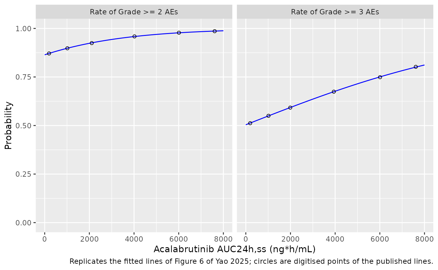
Predicted adverse-event risk in the simulated cohorts
Applying the two regressions to the simulated AUC24h,ss of the two cohorts shows what the 22.6% higher East Asian exposure implies for safety: a difference of about one to two percentage points, consistent with the paper’s conclusion that the higher exposure in Chinese patients is not a safety concern.
auc_sim <- ss |> filter(analyte == "Acalabrutinib", PPTESTCD == "auc24ss")
risk <- auc_sim |>
  mutate(
    p_grade2 = er_eval("Yao_2025_acalabrutinib_teae_grade2", "prob_teae_grade2", value),
    p_grade3 = er_eval("Yao_2025_acalabrutinib_teae_grade3", "prob_teae_grade3", value),
    arm = factor(arm, levels = arms)
  ) |>
  group_by(arm) |>
  summarise(median_auc = median(value), mean_p_grade2 = mean(p_grade2),
            mean_p_grade3 = mean(p_grade3), .groups = "drop")
risk |>
  rename("Cohort" = arm, "Median AUC24h,ss (ng*h/mL)" = median_auc,
         "Mean P(grade >= 2 AE)" = mean_p_grade2,
         "Mean P(grade >= 3 AE)" = mean_p_grade3) |>
knitr::kable(digits = 3, caption = "Predicted adverse-event probability, 100 mg BID.")| Cohort | Median AUC24h,ss (ng*h/mL) | Mean P(grade >= 2 AE) | Mean P(grade >= 3 AE) |
|---|---|---|---|
| Non-East Asian | 1689.917 | 0.918 | 0.584 |
| East Asian | 2071.879 | 0.926 | 0.601 |
Assumptions and deviations
-
Variance scale. Table 3 prints the BSV and BOV
magnitudes with the parameter units (“BSV CL/F (L/h) 23.2”), but the
values are coefficients of variation in percent, as in the Edlund 2022
model that Yao 2025 re-estimates (Edlund 2022: 23.8, 270, 33.7 … CV%).
The maintainers converted each to a log-normal variance with
omega^2 = log(1 + CV^2), the same convention asEdlund_2022_acalabrutinib. -
Covariate form. The Methods give
P = TVP x (1 + Pcov) x exp(eta)for categorical covariates; Table 3 footnote b (“Relative change (1 + estimate)”) is printed on the HEALTHGP, ECOG and PPI rows but not on the EASTASIA rows. The EASTASIA rows use the same form, which the Results confirm (“Vp/F was 38% lower and F was 23% higher”). -
East Asian indicator. EASTASIA covers the 105
Chinese and 6 Japanese patients and is encoded with
RACE_ASIAN_NORTHEAST; no Korean subjects are described in the dataset. The few Asian subjects of the global studies fall in the non-East Asian reference as far as the paper describes. -
Structure carried over. Yao 2025 states that it
used the structure, random-effect models and covariate structure of the
existing global model. The details not repeated in Yao 2025 are taken
from Edlund 2022: the absorption depot between the transit chain and the
central compartment,
ktr = (Ntr + 1) / MTT, the four occasions (three rich occasions plus one lumped sparse occasion, hereOCC1-4; Table 3 footnote a confirms four occasions), and the molar formation of ACP-5862 (formation flux scaled by 481.52 / 465.52 to stay in mg). - F1. Table 3 has no typical F1; F1 is a relative bioavailability fixed at 1 for the reference, carrying the PPI and race effects and BOV.
-
Per-dose BOV in the exposure simulation. Each dose
receives a fresh F1 and MTT draw by changing
etaiov_*_1at every dose onOCC = 1. Users simulating the four analysis occasions should instead supplyOCC1-4. Because rxode2 has no| OCCrandom-effect level, the occasion etas are expanded with indicators; rxode2 therefore warns that these etas are not mu-referenced, which only affects the speed of a future estimation run, not simulation. -
Residual error. The rich and sparse residual SDs
are selected by
SAMPLE_INTENSIVE. Below-LLOQ handling (M3) is an estimation feature and is not part of the model. - Figure 3 comparison. Figure 3 shows empirical-Bayes exposures of the real subjects (with their own PPI and ECOG status and shrunk BOV), so it is not a like-for-like target for a simulated reference cohort; its medians were digitised and serve as an order-of-magnitude check. No published parameter was changed to close the gap.
- Exposure-safety coefficients. No coefficient of the Figure 6 regressions is printed in the paper or its supplement. The intercepts and slopes were recovered from the figure image (a 709 x 341 pixel raster), so they are approximate; the grade >= 2 line runs close to a probability of 1, where the logit is most sensitive to a pixel of error. Neither slope is statistically significant (P = 0.12 and 0.051). The placeholder residual SD of the two logistic models is not from the source; the source likelihood is Bernoulli.
-
Exposure metric.
AUC_ACALABRUTINIBis the parent-drug AUC24h,ss from the post hoc estimates of the population PK model; it can be computed fromYao_2025_acalabrutinibas1000 * daily dose * F1 / CL/F. The ACP-5862 and total-active-moiety exposures of the paper were evaluated only graphically (box plots), as were the exposure-efficacy relationships (Figures 4 and 5); no model was fitted to them. - No erratum or correction notice for the article was found in Europe PMC as of 2026-11-05.