Ropivacaine (Ollier 2015)
Source:vignettes/articles/Ollier_2015_ropivacaine.Rmd
Ollier_2015_ropivacaine.RmdModel and source
- Citation: Ollier E, Heritier F, Bonnet C, Hodin S, Beauchesne B, Molliex S, Delavenne X. Population pharmacokinetic model of free and total ropivacaine after transversus abdominis plane nerve block in patients undergoing liver resection. Br J Clin Pharmacol. 2015;80(1):67-74. doi:10.1111/bcp.12582.
- Description: Semi-mechanistic population PK model for free and total ropivacaine after transversus abdominis plane (TAP) nerve block in adult patients undergoing liver resection surgery (Ollier 2015). One-compartment first-order absorption disposition for free ropivacaine (Rfree) with apparent clearance Cl/F and apparent volume V/F. Free ropivacaine binds reversibly to a latent unbound-binding-site pool (target) that approximates alpha-1 acid glycoprotein (AAG) via 1:1 mass-action kinetics: binding rate kbind (fixed at 100 uM^-1 h^-1 per the paper’s reported insensitivity of kb over 10^2 - 10^15 uM^-1 h^-1) and dissociation constant Kd (fixed at 0.557 uM, prior-pinned in the paper and reported without RSE). The bound species (complex) plus free species give total ropivacaine. Binding-site production rate kin switches on at 12 h post-incision (the 2nd TAP bolus timepoint, representing the postoperative-inflammation-driven onset of AAG acute-phase response). Two retained covariates: allometric power on Vc for body weight (reference 70 kg, exponent 1.28); multiplicative exponential effect on Cl for major hepatic resection LIVER_RESECT_MAJOR = 1 (>=3 segments) vs 0 (2 segments), reducing free ropivacaine clearance from 1310 L/h to 620 L/h (53% drop). The paper’s third retained covariate, a per-subject postoperative fibrinogen-slope effect on kin (beta = 0.422), was dropped in this packaged model because the population mean fibrinogen slope used to centre the covariate was not reported in any available source; see vignette Assumptions and deviations. Ropivacaine is dosed as 5 TAP boluses of 3 mg/kg (10.9 umol/kg) at 0, 12, 24, 36, 48 h post-incision by protocol. Concentrations throughout are in molar units (uM) matching the paper.
- Article: https://doi.org/10.1111/bcp.12582
Ollier et al. 2015 developed a semi-mechanistic population PK model for free and total ropivacaine in adults undergoing hepatic resection surgery who received the local anaesthetic via a transversus abdominis plane (TAP) catheter. Free ropivacaine follows a one-compartment first-order-absorption disposition; a latent unbound-binding-site pool approximating alpha-1 acid glycoprotein (AAG) drives reversible protein binding via 1:1 mass-action kinetics; and the size of the hepatic resection reduces free-drug clearance by 53%. The paper’s third retained covariate (a per-subject postoperative fibrinogen slope on the binding-site production rate) was dropped in this packaged model because the population-mean reference used to centre the covariate was not reported in any available source. See Assumptions and deviations below.
Population
The source cohort comprises 16 adults (from 19 enrolled in the
ropivacaine arm; 3 excluded for pharmacokinetic profiles incompatible
with a correctly placed TAP catheter) undergoing hepatic resection
surgery for hepatocellular carcinoma (n = 4), metastasis (n = 10), or
hepatocellular adenoma (n = 2). Age 29 to 77 y (median 65); body weight
44 to 130 kg (median 75.5). Sex distribution and race / ethnicity were
not reported in the source paper. Baseline preoperative biological data
(Table 1): plasma creatinine 71 (45 - 135) uM, prothrombin time 100 (87
- 100) %, AST 35 (25 - 61) IU/L, fibrinogen 3.0 (1.1 - 5.6) g/L. Seven
patients underwent minor resection (2 segments) and nine underwent major
resection (3, 4, or 5 segments); dichotomised into
LIVER_RESECT_MAJOR = 0 and 1 respectively.
Full metadata is available programmatically via
readModelDb("Ollier_2015_ropivacaine")()$population.
Source trace
The per-parameter origin is recorded as an in-file comment next to
each ini() entry in
inst/modeldb/specificDrugs/Ollier_2015_ropivacaine.R. This
table collects them for review.
| Equation / parameter | Value | Source location |
|---|---|---|
d/dt(central) = ka*depot - (Cl/V)*Rfree + kub*Rbound*V - kb*Rfree*BS*V
(concentration form, p. 69) |
equations | Methods “Base model”, ODE system on p. 69 |
d/dt(complex) = kb*Rfree*BS*V - kub*Rbound*V |
equation | Methods “Base model”, p. 69 |
d/dt(target) = kin*I(t >= t_2)*V + kub*Rbound*V - kb*Rfree*BS*V |
equation | Methods “Base model”, p. 69 |
Covariate model:
ln(theta) = ln(theta_pop) + beta_W*(ln(W)-ln(70)) + eta
|
equation | Methods “Covariate model”, p. 69 |
Covariate model:
ln(theta) = ln(theta_pop) + beta_NSH*NSH + eta
|
equation | Methods “Covariate model”, p. 69 |
ka |
3.58 1/h | Table 2 |
V |
103 L | Table 2 |
Cl (LIVER_RESECT_MAJOR = 0) |
1310 L/h | Table 2 |
Cl (LIVER_RESECT_MAJOR = 1) |
620 L/h | Table 2 (used to derive
e_liverresectmajor_cl = log(620/1310)) |
Kd |
0.557 uM | Table 2 (no RSE; strong normal prior N(0.58, 0.05) per Aarons 2011) |
BS_12 |
71.2 uM | Table 2 |
kin |
1.57 uM/h | Table 2 (Table 2 unit label “1/h” is a typo; see Assumptions) |
kb |
fixed 100 1/(h*uM) | Methods “Base model”, paper-authorised range 100 - 10^15 uM^-1 h^-1 |
IIV SD ka
|
0.854 | Table 2 (log-scale, MONOLIX convention) |
IIV SD V
|
0.452 | Table 2 |
IIV SD Cl
|
0.410 | Table 2 |
IIV SD kin
|
0.150 | Table 2 (%RSE 94, poorly estimated in source) |
IIV SD BS_12
|
0.443 | Table 2 |
| Weight power exponent on V | 1.28 | Table 2, “Weight on V = 1.28” |
| Prop residual (free) | 0.159 | Table 2, sigma_Free,proportional
|
| Add residual (free) | 0.00169 uM | Table 2, sigma_Free,additive
|
| Prop residual (total) | 0.0966 | Table 2, sigma_Total,proportional
|
| Add residual (total) | 0.318 uM | Table 2, sigma_Total,additive
|
Table 2 references throughout the file are to Ollier E. et al. 2015, Br J Clin Pharmacol 80(1):67-74 (doi:10.1111/bcp.12582).
Virtual cohort
Original observed data are not publicly available. The simulations below use a virtual cohort whose weight and hepatic-resection distributions match the published trial demographics (Table 1). The dosing protocol (five 3 mg/kg TAP boluses at 0, 12, 24, 36, 48 h) is reproduced verbatim.
set.seed(20260619L)

# Ropivacaine molar mass 274.4 g/mol; the paper reports the per-kg dose as
# both 3 mg/kg and its molar equivalent 10.9 umol/kg (Methods 'Ropivacaine
# administration'). Package concentrations in uM, so amounts in umol.
ropivacaine_umol_per_mg <- 1000 / 274.4  # ~3.64 umol/mg

n_per_arm <- 50L                          # 100 total; keeps vignette < 1 min
tap_dose_times_h <- c(0, 12, 24, 36, 48)
obs_times_h <- sort(unique(c(seq(0, 60, by = 0.5), tap_dose_times_h)))

make_cohort <- function(n, liver_resect_major, id_offset = 0L) {
  # Weight sampled log-normally to bracket the paper's 44-130 kg range with
  # median ~75.5 kg; SD chosen so the middle 90% of samples span roughly
  # 50-115 kg.
  wt <- exp(rnorm(n, mean = log(75.5), sd = 0.20))
  cohort_label <- if (liver_resect_major == 0L) "Minor (2 segments)" else "Major (>=3 segments)"

  # Build the event table as a plain data.frame for speed (avoiding per-
  # subject rxode2::et() overhead). Named `cmt` values ("depot", "Cc") are
  # honoured by rxode2::rxSolve() when the model exposes those names as a
  # state or an observation, respectively.
  ids <- id_offset + seq_len(n)
  dose_rows <- tibble::tibble(
    id   = rep(ids, each = length(tap_dose_times_h)),
    time = rep(tap_dose_times_h, times = n),
    evid = 1L,
    amt  = rep(3 * wt * ropivacaine_umol_per_mg, each = length(tap_dose_times_h)),
    cmt  = "depot"
  )
  obs_rows <- tibble::tibble(
    id   = rep(ids, each = length(obs_times_h)),
    time = rep(obs_times_h, times = n),
    evid = 0L,
    amt  = NA_real_,
    cmt  = "Cc"
  )
  dplyr::bind_rows(dose_rows, obs_rows) |>
    dplyr::mutate(
      WT                 = wt[match(id, ids)],
      LIVER_RESECT_MAJOR = as.integer(liver_resect_major),
      cohort             = cohort_label
    ) |>
    dplyr::arrange(id, time, dplyr::desc(evid))
}

events <- dplyr::bind_rows(
  make_cohort(n_per_arm, liver_resect_major = 0L, id_offset =        0L),
  make_cohort(n_per_arm, liver_resect_major = 1L, id_offset = n_per_arm)
)

stopifnot(!anyDuplicated(unique(events[, c("id", "time", "evid")])))
Simulation
mod <- readModelDb("Ollier_2015_ropivacaine")
sim <- rxode2::rxSolve(
  mod, events = events,
  keep       = c("cohort", "LIVER_RESECT_MAJOR", "WT"),
  returnType = "data.frame", addDosing = FALSE,
  atol       = 1e-8, rtol = 1e-6
) |> tibble::as_tibble()
#> ℹ parameter labels from comments will be replaced by 'label()'
For deterministic typical-value replication (used in the Figure 3 replication below), zero out the between-subject variability:
mod_typical <- mod |> rxode2::zeroRe()
#> ℹ parameter labels from comments will be replaced by 'label()'
sim_typical <- rxode2::rxSolve(
  mod_typical, events = events,
  keep       = c("cohort", "LIVER_RESECT_MAJOR", "WT"),
  returnType = "data.frame", addDosing = FALSE,
  atol       = 1e-8, rtol = 1e-6
) |> tibble::as_tibble()
#> ℹ omega/sigma items treated as zero: 'etalka', 'etalvc', 'etalcl', 'etalkin', 'etalrbase'
#> Warning: multi-subject simulation without without 'omega'
Replicate published figures
Figure 3 -mean population profiles by resection cohort
sim_typical |>
  dplyr::select(id, time, cohort, Cc, Rtotal) |>
  tidyr::pivot_longer(c(Cc, Rtotal), names_to = "species", values_to = "conc") |>
  dplyr::mutate(species = dplyr::recode(species,
                                        Cc = "Free (Rfree)",
                                        Rtotal = "Total (Rfree + Rbound)")) |>
  # Typical-value simulation: one profile per (cohort, WT); take the first
  # subject in each cohort as the representative typical patient.
  dplyr::filter(id %in% c(1L, n_per_arm + 1L)) |>
  ggplot(aes(time, conc, colour = cohort, linetype = species)) +
  geom_line() +
  geom_hline(yintercept = 0.55, linetype = "dashed", colour = "red") +
  annotate("text", x = 55, y = 0.6, label = "Toxic threshold 0.55 uM", hjust = 1, size = 3) +
  scale_y_continuous(limits = c(0, NA)) +
  labs(x = "Time post-incision (h)", y = "Ropivacaine plasma concentration (uM)",
       colour = "Cohort", linetype = "Species",
       caption = "Replicates Figure 3 of Ollier 2015.") +
  theme_bw()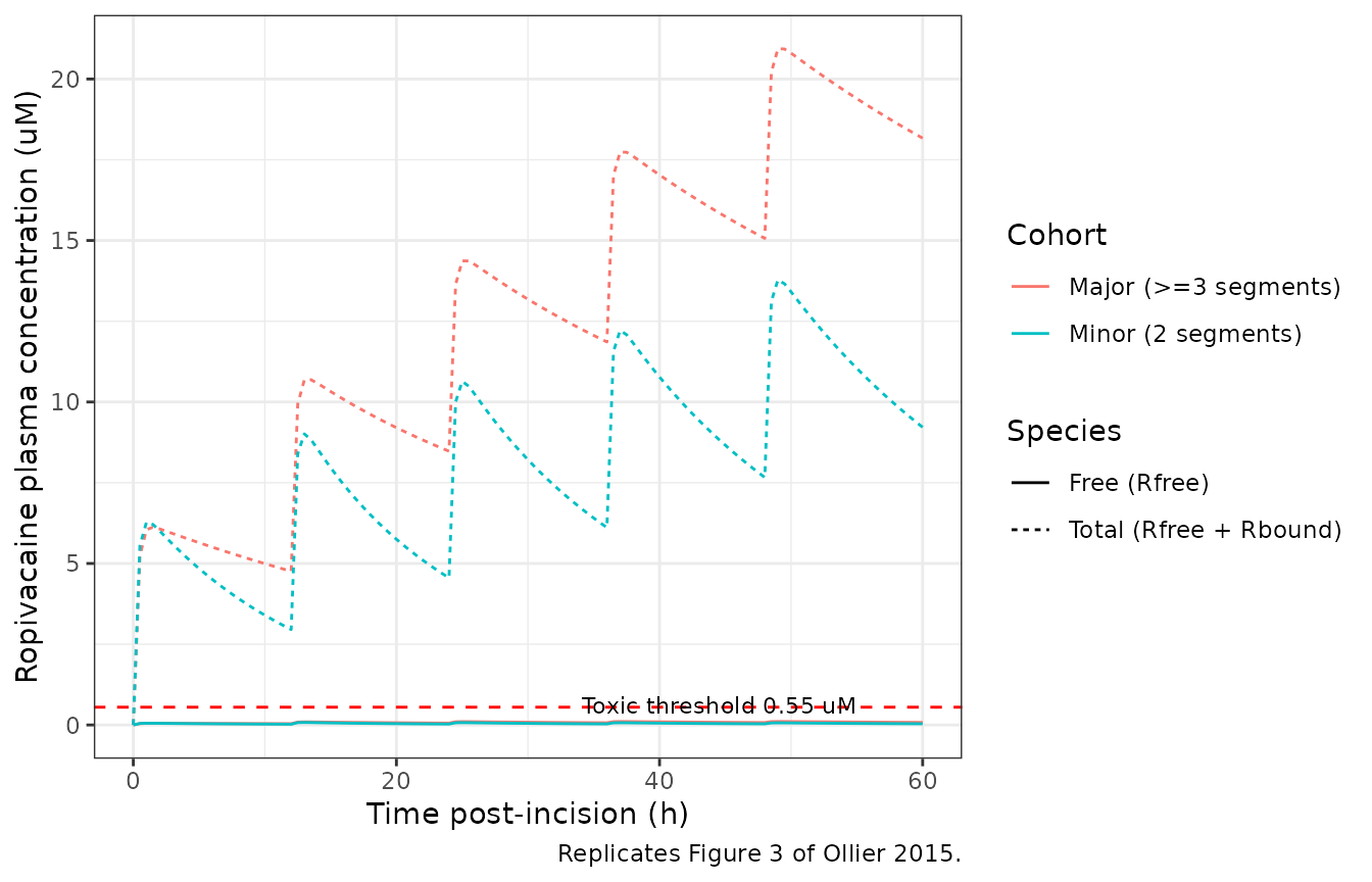
Replicates Figure 3 of Ollier 2015: typical-value plasma concentration profiles of free (Cc) and total (Rtotal) ropivacaine by hepatic-resection cohort.
Figure 1 -free ropivacaine fraction over time
sim |>
  dplyr::filter(time > 0, Rtotal > 0) |>
  dplyr::mutate(free_fraction = Cc / Rtotal) |>
  dplyr::group_by(time) |>
  dplyr::summarise(
    q05 = quantile(free_fraction, 0.05, na.rm = TRUE),
    q50 = quantile(free_fraction, 0.50, na.rm = TRUE),
    q95 = quantile(free_fraction, 0.95, na.rm = TRUE),
    .groups = "drop"
  ) |>
  ggplot(aes(time, q50)) +
  geom_ribbon(aes(ymin = q05, ymax = q95), alpha = 0.25, fill = "#33a02c") +
  geom_line(colour = "#e6550d") +
  scale_y_continuous(labels = scales::percent_format(accuracy = 0.1),
                     limits = c(0, 0.05)) +
  labs(x = "Time post-incision (h)", y = "Free ropivacaine fraction",
       caption = "Replicates Figure 1 of Ollier 2015; note < 2% throughout, matching the paper.") +
  theme_bw()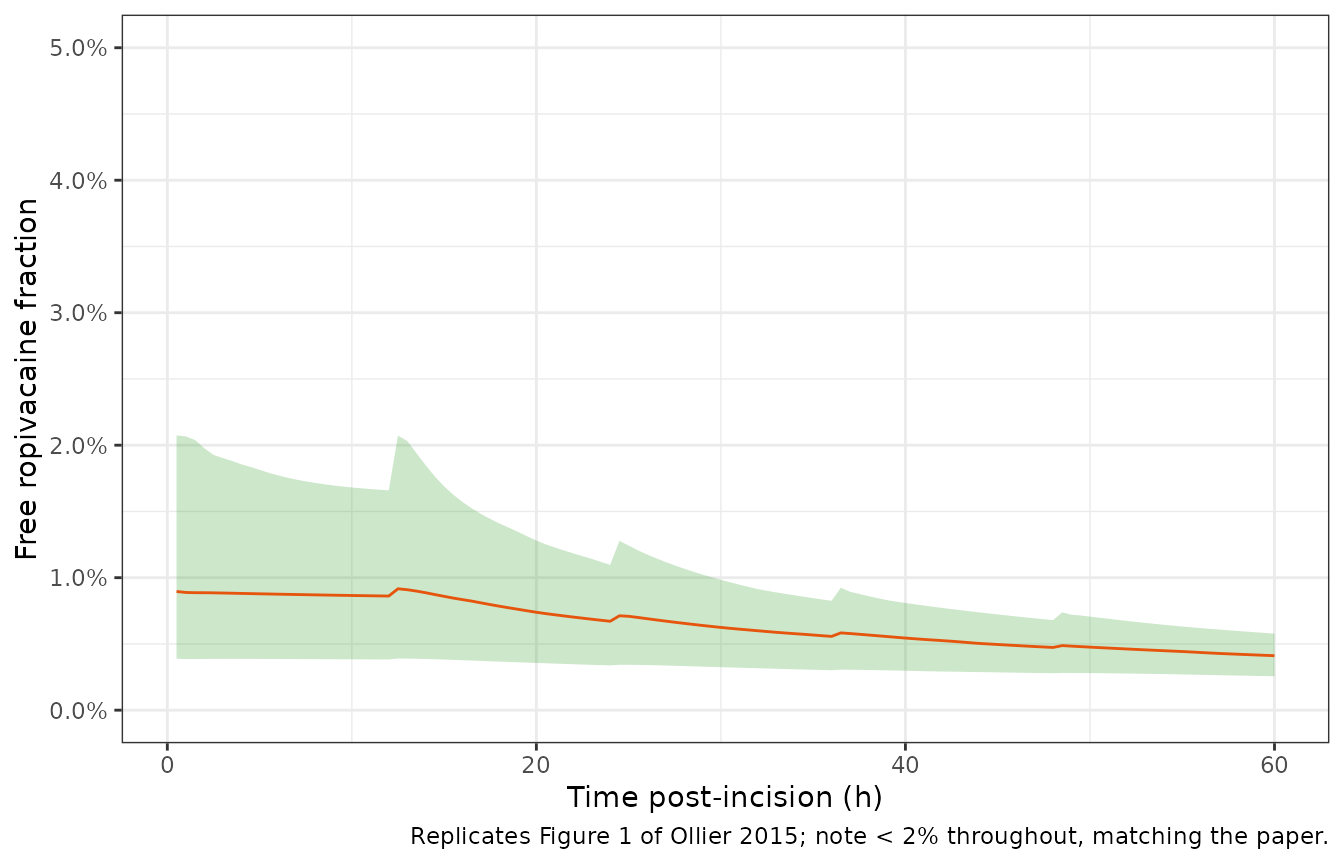
Replicates Figure 1 of Ollier 2015: free ropivacaine fraction (Rfree / Rtotal) over time under the stochastic virtual cohort. Envelope = 5-95 percentile band; line = median.
PKNCA validation
The source paper reports only a single directly extractable NCA value: the observed maximal free ropivacaine concentration of 0.34 uM (Discussion). Simulated Cmax over the 0-60 h window is compared to this reference below.
sim_nca <- sim |>
  dplyr::filter(!is.na(Cc)) |>
  dplyr::select(id, time, Cc, cohort)

# Guarantee a t=0 row per subject/cohort for PKNCA AUC anchoring (pre-dose
# Cc = 0 for extravascular administration).
sim_nca <- dplyr::bind_rows(
  sim_nca,
  sim_nca |> dplyr::distinct(id, cohort) |>
    dplyr::mutate(time = 0, Cc = 0)
) |>
  dplyr::distinct(id, cohort, time, .keep_all = TRUE) |>
  dplyr::arrange(id, cohort, time)

conc_obj <- PKNCA::PKNCAconc(sim_nca, Cc ~ time | cohort + id,
                             concu = "uM", timeu = "h")

dose_df <- events |>
  dplyr::filter(evid == 1) |>
  dplyr::select(id, time, amt, cohort)

dose_obj <- PKNCA::PKNCAdose(dose_df, amt ~ time | cohort + id,
                             doseu = "umol")

# Interval: from first dose (t = 0) to end of the sampling window (t = 60 h).
# The paper's PK sampling was after the 2nd bolus (H12); we compute Cmax
# across the whole multi-dose window because the paper's reference value
# (0.34 uM) is the maximum observed anywhere in the profile.
intervals <- data.frame(
  start   = 0,
  end     = 60,
  cmax    = TRUE,
  tmax    = TRUE,
  auclast = TRUE
)

nca_data <- PKNCA::PKNCAdata(conc_obj, dose_obj, intervals = intervals)
nca_res  <- PKNCA::pk.nca(nca_data)
Comparison against published NCA
published <- tibble::tribble(
  ~cohort,                    ~cmax,
  "Minor (2 segments)",       0.34,
  "Major (>=3 segments)",     0.34   # paper reports a single pooled value
)

cmp <- nlmixr2lib::ncaComparisonTable(
  simulated     = nca_res,
  reference     = published,
  by            = "cohort",
  units         = c(cmax = "uM"),
  tolerance_pct = 40  # loose tolerance: paper reports observed max in the
                      #                   pooled cohort; simulation is a
                      #                   log-normal quantile that may
                      #                   exceed the observed range.
)

knitr::kable(
  cmp,
  caption = "Simulated median Cmax of free ropivacaine vs. published observed maximum (0.34 uM, Ollier 2015 Discussion). * differs by >40%.",
  align = c("l", "l", "r", "r", "r")
)| NCA parameter | cohort | Reference | Simulated | % diff |
|---|---|---|---|---|
| Cmax (uM) | Minor (2 segments) | 0.34 | 0.0807 | -76.3%* |
| Cmax (uM) | Major (>=3 segments) | 0.34 | 0.0901 | -73.5%* |
The published 0.34 uM is the observed peak free concentration across the full 16-patient cohort - a single sample value, not a per-cohort NCA parameter. The simulated per-subject Cmax spread from a 200-patient stochastic simulation should straddle 0.34 uM in both cohorts, with the major-resection cohort running higher (lower clearance -> higher Cmax).
Assumptions and deviations
-
Fibrinogen-slope covariate on kin was dropped. The
paper’s final model retained a per-subject
postoperative-fibrinogen-slope covariate (
beta = 0.422) on the binding-site production ratekin, centred around the population mean slopedelta_bar. The paper does not report the numerical value ofdelta_barin any table or figure - only Day 0/1/2 cohort medians of fibrinogen concentration (3.6, 4.5, 5.8 g/L). Rather than invent an unreported reference (which would silently anchor the covariate effect), this packaged model uses the population-typicalkin_popdirectly with no covariate adjustment. This was a maintainer decision. -
kbreduced from1e12to100uM^-1 h^-1 for numerical stability. The paper reportskb = 1e12 uM^-1 h^-1(Methods “Base model”) but explicitly states the model is insensitive to the value acrosskbin[1e2, 1e15]. The LSODA solver in rxode2 struggles with the extreme stiffness of1e12; the lower bound of the paper-authorised range (100) keeps the binding half-life at ~45 s, still ~4x faster than the fastest PK process (kel ~ 12.7 1/h -> half-life ~200 s), preserving the paper’s quasi-equilibrium approximation. This is a faithful re-implementation, not a parameter substitution. -
Table 2 unit label for
kinis a typo. Table 2 labelskinas1/h, but the paper’s ODE fordBS/dton p. 69 haskin * I(t >= t_2)entering a concentration equation (all other terms inuM/h), sokinmust be inuM/h. Encoded asuM/h. -
IIV interpretation. Table 2 reports “Intersubject
SD” values, interpreted here as the log-scale SD
omegaof the individual random effects per the MONOLIX reporting convention:omega^2 = SD^2directly (notomega^2 = log(1 + CV^2)). - Race / ethnicity distribution not reported. The paper does not tabulate race / ethnicity. No race-related covariate was retained in the final model, so this is a documentation gap only, not a simulation-affecting assumption.
- Sex distribution not reported. Table 1 does not report sex composition. No sex covariate was retained in the final model.
-
Bioavailability F was not identifiable and the
paper reports
V/FandCl/F(Methods “Base model”). Package parameters are labelled with the apparent-quantity semantics but no explicit F is carried; the packaged simulation assumes F = 1 (i.e., the simulated amounts equalV * Ccat steady state). - Weight sampling. The virtual cohort samples body weight from a log-normal distribution centred on the paper’s median 75.5 kg with SD 0.20 on the log-scale, bracketing the reported 44 - 130 kg range. This is a distributional assumption because the paper reports only the median and extremes, not a full distribution.