Donepezil oral and long-acting intramuscular GB-5001 (Khwarg 2024)
Source:vignettes/articles/Khwarg_2024_donepezil.Rmd
Khwarg_2024_donepezil.RmdModel and source
Khwarg 2024 developed a single NONMEM population PK analysis of donepezil covering two formulations: the marketed oral tablet (Aricept 10 mg) and GB-5001, a long-acting intramuscular (IM) depot injection under development for Alzheimer’s disease. Because the authors estimated clearance, both volumes, inter-compartmental clearance and the residual-error model separately for each formulation, the two arms share no parameters and are distributed here as two model files that point at this one article.
mod_oral <- readModelDb("Khwarg_2024_donepezil_oral")
mod_im <- readModelDb("Khwarg_2024_donepezil_im")- Oral: Two-compartment population PK model for oral donepezil (Aricept 10 mg tablet) with first-order absorption and an absorption lag time, in healthy adult men
- IM: Two-compartment population PK model for long-acting intramuscular donepezil (GB-5001) with three-phase absorption: two lagged parallel first-order depots plus a simultaneous zero-order input, in healthy adult men
- Citation: Khwarg J, Lee H, Yu KS, Seol E, Chung JY. Population Pharmacokinetic Modeling and Simulation for Dose Optimization of GB-5001, a Long-Acting Intramuscular Injection of Donepezil, in Healthy Participants. Neurol Ther. 2024;13(5):1453-1466. doi:10.1007/s40120-024-00643-4. Companion intramuscular model: modellib(‘Khwarg_2024_donepezil_im’).
- Article: https://doi.org/10.1007/s40120-024-00643-4
- Trial registration: NCT05525780
Population
The models were fitted to plasma donepezil concentrations from a randomized, double-blind, placebo-controlled phase 1 dose-escalation study in 48 healthy non-smoking men aged 18-55 years with a BMI of 18.5-30.0 kg/m2 (Khwarg 2024, “Study Participants” and “Demographics”).
Participants were assigned to four cohorts of 12. Cohorts 1-3 received a single gluteal IM injection of GB-5001 at 70, 140 or 280 mg, randomized 3:1 against a matching placebo, so 9 participants per dose level (27 in total) contributed donepezil concentrations. Cohort 4 received a single 10 mg oral Aricept tablet; all 12 contributed concentrations. IM-cohort participants were 94.4% white with mean age 39.9 (SD 9.8) years and mean weight 78.7 (SD 7.3) kg; the oral cohort was 100% white with mean age 39.5 (SD 10.2) years and mean weight 82.4 (SD 9.1) kg. No covariate effects were retained in the final model.
The same information is available programmatically via each model’s
population metadata,
e.g. readModelDb("Khwarg_2024_donepezil_im")()$population.
Source trace
Every ini() entry in both model files carries an in-file
comment naming its source location. They are collected here for review.
All parameter values come from Khwarg 2024 Table 2 (“Parameter estimates
of the population pharmacokinetic model of donepezil for oral and
intramuscular formulation”), final-model estimate column; the model
topology comes from Figure 2.
| Model | Equation / parameter | Value | Source location |
|---|---|---|---|
| both | Two-compartment disposition, formulation-specific absorption | n/a | Fig. 2 (structural diagram) |
| oral |
lka (KA, depot 1) |
0.203 1/h | Table 2, Oral block |
| oral |
lcl (CL) |
14.3 L/h | Table 2, Oral block |
| oral |
lvc (V2) |
39.5 L | Table 2, Oral block |
| oral |
lq (Q) |
84.9 L/h | Table 2, Oral block |
| oral |
lvp (V3) |
1080 L | Table 2, Oral block |
| oral |
ltlag (ALAG1) |
0.931 h | Table 2, Oral block |
| oral |
lfdepot (F1) |
1, fixed | Table 2, Oral block; anchored to the high oral bioavailability of Aricept (ref [14]) |
| oral |
etalcl + etalvc block |
0.0475 / -0.144 / 1.59 | Table 2, Oral block (22.1%, -52.0%, 197.6%) |
| oral | etalvp |
0.0153 | Table 2, Oral block (12.4%) |
| oral | etalfdepot |
0.0162 | Table 2, Oral block (12.8%) |
| oral |
propSd / addSd
|
0.137 / 0.138 ug/L | Table 2, Oral block (additive reported as 138 pg/mL) |
| IM |
lfdepot (F4) |
0.748 | Table 2, Intramuscular block |
| IM |
lfdepot2 (F5) |
0.145 | Table 2, Intramuscular block |
| IM | zero-order fraction 1 - F4 - F5
|
0.107 | Fig. 2 (labelled “1-F4-F5” on the zero-order arm) |
| IM |
lka (KA4, depot 4) |
0.00402 1/h | Table 2, Intramuscular block |
| IM |
lka2 (KA5, depot 5) |
0.0134 1/h | Table 2, Intramuscular block |
| IM |
ltlag (ALAG4) |
235 h | Table 2, Intramuscular block |
| IM |
ltlag2 (ALAG5) |
645 h | Table 2, Intramuscular block |
| IM |
ld1 (D2, zero-order duration) |
648 h | Table 2, Intramuscular block |
| IM |
lcl (CL) |
10.3 L/h | Table 2, Intramuscular block |
| IM |
lvc (V2) |
503 L | Table 2, Intramuscular block |
| IM |
lq (Q) |
185 L/h | Table 2, Intramuscular block |
| IM |
lvp (V3) |
1160 L | Table 2, Intramuscular block |
| IM |
etalcl + etalvc block |
0.0936 / 0.113 / 1.13 | Table 2, Intramuscular block (31.3%, 144.8%) |
| IM |
propSd / addSd
|
0.223 / 0.0235 ug/L | Table 2, Intramuscular block (additive reported as 23.5 pg/mL) |
Two transcription notes:
- The text extraction from the source PDF dropped the
KA5row of Table 2 entirely. The value used here (0.0134 1/h, RSE 17.2%) was read from the raw PDF, where the row sits betweenKA4and the IMCLrow. - Table 2 reports IIV as the log-scale variance; the
parenthesised percentage is the derived CV via footnote b,
CV = sqrt(exp(omega^2) - 1) * 100. Each value was checked against its own footnote (e.g.sqrt(exp(0.0475) - 1) = 22.1%) before being used directly as a variance. Both OMEGA blocks are positive definite as published.
Encoding the three-phase IM absorption
Figure 2 splits each IM dose three ways. In rxode2 this is expressed
with one dose record per arm, all carrying the full nominal
dose, with the f() multipliers performing the
split:
| Arm | cmt |
rate |
Fraction | Control |
|---|---|---|---|---|
| First-order depot | depot |
0 | F4 = 0.748 |
alag(depot) = 235 h, ka = 0.00402 1/h
|
| First-order depot | depot2 |
0 | F5 = 0.145 |
alag(depot2) = 645 h,
ka2 = 0.0134 1/h
|
| Zero-order input | central |
-2 | 1 - F4 - F5 = 0.107 | dur(central) = 648 h |
rate = -2 tells rxode2 that the infusion duration is
supplied by the model (dur(central)) rather than by the
data.
Virtual cohort
Original observed data are not publicly available. The simulations below use virtual cohorts of 100 participants per arm, dosed and sampled at the study’s published nominal times (Khwarg 2024, “Clinical Study Design”) so that the simulated NCA is directly comparable with the paper’s own NCA in Table 1.
set.seed(20240810)

im_times <- c(0, 0.5, 1, 2, 4, 6, 8, 12, 24, 48, 72, 96, 120, 168, 240, 312,
              360, 432, 504, 552, 600, 648, 720, 768, 840, 1008, 1176, 1512)
oral_times <- c(0, 0.5, 1, 1.5, 2, 2.5, 3, 3.5, 4, 4.5, 6, 8, 12, 24, 48, 96,
                120, 144, 240)

# The IM dose is split across three parallel records (see the table above); each
# record carries the full nominal dose because f() applies the fraction.
make_im_events <- function(dose, n, obs_times, dose_times, treatment, id_offset = 0L) {
  ids <- id_offset + seq_len(n)
  doses <- tidyr::expand_grid(
    id = ids,
    time = dose_times,
    tibble::tibble(cmt = c("depot", "depot2", "central"), rate = c(0, 0, -2))
  ) |>
    dplyr::mutate(amt = dose, evid = 1L)
  obs <- tidyr::expand_grid(id = ids, time = obs_times) |>
    dplyr::mutate(amt = NA_real_, evid = 0L, cmt = "central", rate = 0)
  dplyr::bind_rows(doses, obs) |>
    dplyr::mutate(treatment = treatment, nominal_dose = dose) |>
    dplyr::arrange(id, time, dplyr::desc(evid))
}

make_oral_events <- function(dose, n, obs_times, dose_times, treatment, id_offset = 0L) {
  ids <- id_offset + seq_len(n)
  doses <- tidyr::expand_grid(id = ids, time = dose_times) |>
    dplyr::mutate(amt = dose, evid = 1L, cmt = "depot", rate = 0)
  obs <- tidyr::expand_grid(id = ids, time = obs_times) |>
    dplyr::mutate(amt = NA_real_, evid = 0L, cmt = "central", rate = 0)
  dplyr::bind_rows(doses, obs) |>
    dplyr::mutate(treatment = treatment, nominal_dose = dose) |>
    dplyr::arrange(id, time, dplyr::desc(evid))
}

n_arm <- 100

ev_im <- dplyr::bind_rows(
  make_im_events(70,  n_arm, im_times, 0, "IM 70 mg",  id_offset =   0L),
  make_im_events(140, n_arm, im_times, 0, "IM 140 mg", id_offset = 100L),
  make_im_events(280, n_arm, im_times, 0, "IM 280 mg", id_offset = 200L)
)
ev_oral <- make_oral_events(10, n_arm, oral_times, 0, "Oral 10 mg", id_offset = 300L)

stopifnot(
  # No record collides with another on the (subject, time, type, compartment) key.
  anyDuplicated(ev_im[, c("id", "time", "evid", "cmt")]) == 0L,
  anyDuplicated(ev_oral[, c("id", "time", "evid", "cmt")]) == 0L,
  # Three dose records per IM administration (one per absorption arm), one per
  # oral administration.
  sum(ev_im$evid == 1L) == 3L * 3L * n_arm,
  sum(ev_oral$evid == 1L) == n_arm,
  # Every IM dose record carries the full nominal dose; f() performs the split.
  all(ev_im$amt[ev_im$evid == 1L] == ev_im$nominal_dose[ev_im$evid == 1L])
)
Simulation
The two formulations are solved with their own model. Grouping labels
ride through rxSolve(keep = ...) rather than a post-hoc
join.
sim_im <- rxode2::rxSolve(mod_im, events = ev_im,
                          keep = c("treatment", "nominal_dose")) |>
  as.data.frame()
#> ℹ parameter labels from comments will be replaced by 'label()'
sim_oral <- rxode2::rxSolve(mod_oral, events = ev_oral,
                            keep = c("treatment", "nominal_dose")) |>
  as.data.frame()
#> ℹ parameter labels from comments will be replaced by 'label()'

sim <- dplyr::bind_rows(sim_im, sim_oral) |>
  dplyr::mutate(treatment = factor(
    treatment,
    levels = c("IM 70 mg", "IM 140 mg", "IM 280 mg", "Oral 10 mg")
  ))

# rxSolve silently drops subjects on solver failure; assert the count.
stopifnot(dplyr::n_distinct(sim$id) == 4 * n_arm)
Replicate published figures
Figure 1 – mean plasma concentration-time profiles
# Replicates Figure 1A of Khwarg 2024: mean plasma donepezil after a single IM
# dose of GB-5001 at 70, 140 and 280 mg, linear scale.
sim |>
  dplyr::filter(grepl("^IM", treatment)) |>
  dplyr::group_by(treatment, time) |>
  dplyr::summarise(mean_Cc = mean(Cc), .groups = "drop") |>
  ggplot(aes(time, mean_Cc, colour = treatment)) +
  geom_line() +
  geom_point(size = 0.8) +
  labs(x = "Time (h)", y = "Mean donepezil concentration (ug/L)",
       colour = NULL,
       title = "Figure 1A -- IM GB-5001, single dose",
       caption = "Replicates Figure 1A of Khwarg 2024.") +
  theme(legend.position = "bottom")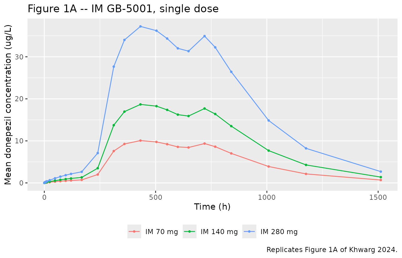
The simulated IM profiles reproduce the two features the paper highlights: a slow, low-level rise beginning immediately after injection (the zero-order arm, which runs for 648 h with no lag), and a double peak produced by the two lagged first-order depots switching on at 235 h and 645 h.
# Locate the local maxima of the typical-value 280 mg profile.
mod_im_typ <- rxode2::zeroRe(mod_im)
#> ℹ parameter labels from comments will be replaced by 'label()'
prof <- rxode2::rxSolve(
  mod_im_typ,
  make_im_events(280, 1, seq(0, 1512, by = 2), 0, "IM 280 mg"),
  keep = "treatment"
) |>
  as.data.frame() |>
  dplyr::filter(time > 0)
#> ℹ omega/sigma items treated as zero: 'etalcl', 'etalvc'

peaks <- prof$time[which(diff(sign(diff(prof$Cc))) < 0) + 1]
peaks
#> [1] 434 698
# Replicates Figure 1B of Khwarg 2024: mean plasma donepezil after a single
# 10 mg oral Aricept tablet, linear scale.
sim |>
  dplyr::filter(treatment == "Oral 10 mg") |>
  dplyr::group_by(time) |>
  dplyr::summarise(mean_Cc = mean(Cc), .groups = "drop") |>
  ggplot(aes(time, mean_Cc)) +
  geom_line() +
  geom_point(size = 0.8) +
  labs(x = "Time (h)", y = "Mean donepezil concentration (ug/L)",
       title = "Figure 1B -- oral Aricept 10 mg, single dose",
       caption = "Replicates Figure 1B of Khwarg 2024.")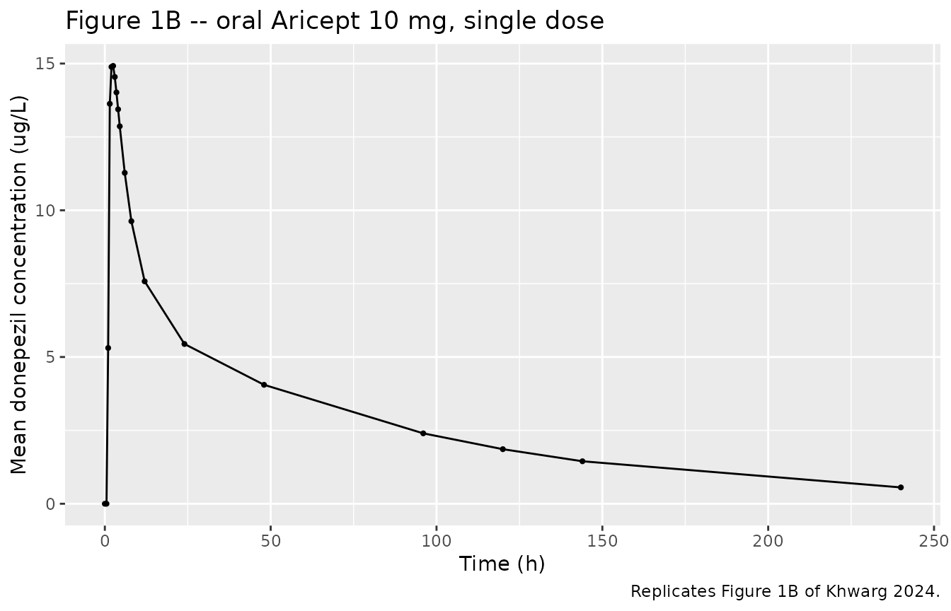
Figure 2 – decomposing the three IM absorption arms
Not a figure the paper plots numerically, but a direct check that the encoded dose split matches the Figure 2 diagram: simulating each arm in isolation shows which part of the profile it contributes.
arm_profile <- function(keep_arm) {
  ev <- make_im_events(280, 1, seq(0, 1512, by = 4), 0, "IM 280 mg") |>
    dplyr::filter(evid == 0 | cmt == keep_arm)
  rxode2::rxSolve(mod_im_typ, ev, keep = "treatment") |>
    as.data.frame() |>
    dplyr::transmute(time, Cc, arm = keep_arm)
}

dplyr::bind_rows(
  arm_profile("depot")   |> dplyr::mutate(arm = "First-order depot (F4, lag 235 h)"),
  arm_profile("depot2")  |> dplyr::mutate(arm = "First-order depot2 (F5, lag 645 h)"),
  arm_profile("central") |> dplyr::mutate(arm = "Zero-order into central (1-F4-F5, D2 = 648 h)")
) |>
  ggplot(aes(time, Cc, colour = arm)) +
  geom_line() +
  labs(x = "Time (h)", y = "Donepezil concentration (ug/L)", colour = NULL,
       title = "Contribution of each IM absorption arm (280 mg, typical values)",
       caption = "Decomposition of the Figure 2 structural model.") +
  theme(legend.position = "bottom", legend.direction = "vertical")
#> ℹ omega/sigma items treated as zero: 'etalcl', 'etalvc'
#> ℹ omega/sigma items treated as zero: 'etalcl', 'etalvc'
#> ℹ omega/sigma items treated as zero: 'etalcl', 'etalvc'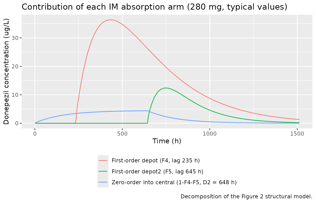
PKNCA validation
sim_nca <- sim |>
  dplyr::filter(!is.na(Cc)) |>
  # `treatment` is a factor in `sim` for plot ordering, but `dose_df` below
  # carries it as character; PKNCA groups must agree in type across the conc
  # and dose objects, so drop back to character here.
  dplyr::mutate(treatment = as.character(treatment)) |>
  dplyr::select(id, time, Cc, treatment)

# Guarantee a time = 0 row per subject; donepezil is extravascular in both
# formulations, so pre-dose Cc = 0 is the correct anchor for AUC0-*.
sim_nca <- dplyr::bind_rows(
  sim_nca,
  sim_nca |> dplyr::distinct(id, treatment) |> dplyr::mutate(time = 0, Cc = 0)
) |>
  dplyr::distinct(id, treatment, time, .keep_all = TRUE) |>
  dplyr::arrange(id, treatment, time)

conc_obj <- PKNCA::PKNCAconc(sim_nca, Cc ~ time | treatment + id,
                             concu = "ug/L", timeu = "h")

# IMPORTANT: the IM event table carries THREE dose records per administration
# (one per absorption arm), each holding the full nominal dose because f()
# performs the split. Filtering `evid == 1` would hand PKNCA three times the
# administered dose and inflate CL/F and Vz/F threefold. Build the dose frame
# from the nominal dose instead: one row per subject per administration.
#
# PKNCA derives CL/F as dose / AUCinf and Vz/F as dose / (lambda.z * AUCinf), so
# the dose must carry the same mass unit as the concentration numerator. The
# simulated concentrations are ug/L while the doses are nominally mg, so the
# dose is converted to ug here; otherwise both parameters come out 1000-fold
# too small (mg/(h*ug/L) rather than L/h).
dose_df <- dplyr::bind_rows(ev_im, ev_oral) |>
  dplyr::filter(evid == 1) |>
  dplyr::distinct(id, time, treatment, nominal_dose) |>
  dplyr::mutate(amt = nominal_dose * 1000) |>
  dplyr::select(-nominal_dose)

stopifnot(nrow(dose_df) == 4 * n_arm)

dose_obj <- PKNCA::PKNCAdose(dose_df, amt ~ time | treatment + id, doseu = "ug")

intervals <- data.frame(
  start      = 0,
  end        = Inf,
  cmax       = TRUE,
  tmax       = TRUE,
  auclast    = TRUE,
  aucinf.obs = TRUE,
  half.life  = TRUE,
  cl.obs     = TRUE,
  vz.obs     = TRUE
)

nca_res <- PKNCA::pk.nca(PKNCA::PKNCAdata(conc_obj, dose_obj, intervals = intervals))
Comparison against published NCA
Khwarg 2024 Table 1 reports arithmetic mean (SD) NCA parameters per
arm. Note that the paper’s AUCt, CL/F and
Vd/F correspond to PKNCA’s auclast,
cl.obs and vz.obs, and that the paper’s
concentration unit (ug/L) equals ng/mL. cl.obs and
vz.obs are reported in L/h and L because the dose handed to
PKNCAdose() above was converted to ug to match the ug/L
concentration scale.
published <- tibble::tribble(
  ~treatment,    ~cmax,  ~tmax, ~auclast, ~aucinf.obs, ~half.life, ~cl.obs, ~vz.obs,
  "IM 70 mg",    11.98,  432,    6800,     6900,        170,        11,      2700,
  "IM 140 mg",   24.43,  434,   15000,    15000,        150,        11,      2300,
  "IM 280 mg",   47.63,  433,   29000,    30000,        190,        11,      2700,
  "Oral 10 mg",  18.02,    2.25,  670,      770,         88,        14,      1600
)

cmp <- nlmixr2lib::ncaComparisonTable(
  simulated = nca_res,
  reference = published,
  by        = "treatment",
  units     = c(cmax = "ug/L", tmax = "h", auclast = "h*ug/L",
                aucinf.obs = "h*ug/L", half.life = "h",
                cl.obs = "L/h", vz.obs = "L"),
  tolerance_pct = 20
)

knitr::kable(
  cmp,
  caption = "Simulated vs. published NCA (Khwarg 2024 Table 1). * differs from reference by >20%.",
  digits = 3
)| NCA parameter | treatment | Reference | Simulated | % diff |
|---|---|---|---|---|
| Cmax (ug/L) | IM 70 mg | 12 | 10.4 | -13.5% |
| Cmax (ug/L) | IM 140 mg | 24.4 | 18.7 | -23.3%* |
| Cmax (ug/L) | IM 280 mg | 47.6 | 38 | -20.2%* |
| Cmax (ug/L) | Oral 10 mg | 18 | 16.1 | -10.7% |
| Tmax (h) | IM 70 mg | 432 | 432 | +0.0% |
| Tmax (h) | IM 140 mg | 434 | 432 | -0.5% |
| Tmax (h) | IM 280 mg | 433 | 432 | -0.2% |
| Tmax (h) | Oral 10 mg | 2.25 | 2 | -11.1% |
| AUC0-∞ (obs) (h*ug/L) | IM 70 mg | 6900 | 6950 | +0.8% |
| AUC0-∞ (obs) (h*ug/L) | IM 140 mg | 15000 | 12400 | -17.2% |
| AUC0-∞ (obs) (h*ug/L) | IM 280 mg | 30000 | 25900 | -13.8% |
| AUC0-∞ (obs) (h*ug/L) | Oral 10 mg | 770 | 680 | -11.7% |
| AUClast (h*ug/L) | IM 70 mg | 6800 | 6790 | -0.2% |
| AUClast (h*ug/L) | IM 140 mg | 15000 | 12300 | -18.1% |
| AUClast (h*ug/L) | IM 280 mg | 29000 | 25100 | -13.4% |
| AUClast (h*ug/L) | Oral 10 mg | 670 | 627 | -6.4% |
| t½ (h) | IM 70 mg | 170 | 162 | -4.9% |
| t½ (h) | IM 140 mg | 150 | 167 | +11.2% |
| t½ (h) | IM 280 mg | 190 | 168 | -11.5% |
| t½ (h) | Oral 10 mg | 88 | 63.2 | -28.2%* |
| CL/F (L/h) | IM 70 mg | 11 | 10.1 | -8.5% |
| CL/F (L/h) | IM 140 mg | 11 | 11.3 | +2.4% |
| CL/F (L/h) | IM 280 mg | 11 | 10.8 | -1.5% |
| CL/F (L/h) | Oral 10 mg | 14 | 14.7 | +5.0% |
| Vz/F (L) | IM 70 mg | 2700 | 2400 | -11.1% |
| Vz/F (L) | IM 140 mg | 2300 | 2760 | +19.8% |
| Vz/F (L) | IM 280 mg | 2700 | 2670 | -1.1% |
| Vz/F (L) | Oral 10 mg | 1600 | 1350 | -15.6% |
- differs from reference by more than ±20%.
Mass-balance check on the IM dose split
The three IM arms partition the dose into F4 + F5 + (1 - F4 - F5) =
1, so the IM formulation is implicitly fully bioavailable and
AUCinf must equal Dose / CL exactly.
Confirming this validates the dose split, the units, and the IM
clearance in one step.
tibble::tibble(dose_mg = c(70, 140, 280)) |>
  dplyr::mutate(
    `AUCinf from Dose/CL (h*ug/L)` = dose_mg / 10.3 * 1000,
    `Published AUCinf (h*ug/L)`    = c(6900, 15000, 30000)
  ) |>
  dplyr::rename("IM dose (mg)" = dose_mg) |>
knitr::kable(digits = 0, caption = "IM AUCinf implied by Dose/CL vs Khwarg 2024 Table 1.")| IM dose (mg) | AUCinf from Dose/CL (h*ug/L) | Published AUCinf (h*ug/L) |
|---|---|---|
| 70 | 6796 | 6900 |
| 140 | 13592 | 15000 |
| 280 | 27184 | 30000 |
Dose proportionality of the typical-value IM profile
The three starred rows in the table above are all Cmax
(IM 140 and 280 mg) and the oral half-life. To separate a model defect
from cohort sampling noise, the check below drops the random effects
entirely: a linear model must give an exactly dose-proportional
typical-value profile, and the paper’s own power-model analysis
concluded the IM formulation is dose-proportional over 70-280 mg (slope
1.043, 90% CI 0.842-1.245).
typ_profile <- function(dose) {
  ev <- make_im_events(dose, 1, seq(0, 1512, by = 1), 0, paste0("IM ", dose, " mg"))
  s <- as.data.frame(rxode2::rxSolve(mod_im_typ, ev, keep = "treatment"))
  s <- s[!is.na(s$Cc), ]
  tibble::tibble(
    `IM dose (mg)`         = dose,
    `Typical Cmax (ug/L)`  = max(s$Cc),
    `Cmax per mg`          = max(s$Cc) / dose,
    `Typical Tmax (h)`     = s$time[which.max(s$Cc)],
    `Published Cmax per mg` = c(11.98, 24.43, 47.63)[match(dose, c(70, 140, 280))] / dose
  )
}

dplyr::bind_rows(lapply(c(70, 140, 280), typ_profile)) |>
  knitr::kable(digits = 4,
               caption = "Typical-value (zeroRe) IM profile: dose proportionality and Tmax.")
#> ℹ omega/sigma items treated as zero: 'etalcl', 'etalvc'
#> ℹ omega/sigma items treated as zero: 'etalcl', 'etalvc'
#> ℹ omega/sigma items treated as zero: 'etalcl', 'etalvc'| IM dose (mg) | Typical Cmax (ug/L) | Cmax per mg | Typical Tmax (h) | Published Cmax per mg |
|---|---|---|---|---|
| 70 | 10.1277 | 0.1447 | 434 | 0.1711 |
| 140 | 20.2553 | 0.1447 | 434 | 0.1745 |
| 280 | 40.5106 | 0.1447 | 434 | 0.1701 |
Cmax per mg is identical to four decimal places across
the three doses and Tmax is 434 h at every dose, against a
published median Tmax of 432-434 h. The model therefore
reproduces the paper’s dose proportionality and its absorption timing
exactly; the residual Cmax gap is a level offset of about
15% against the observed arithmetic means, discussed below.
Bioequivalence simulation (Figure 5)
The paper’s headline result is a dose-optimization exercise: which IM dose of GB-5001, given every 4 weeks, is bioequivalent to 10 mg oral donepezil once daily? The published design simulates a parallel-group trial of oral 10 mg once daily for 28 days against IM doses of 185-225 mg (5 mg increments) given three times at 4-week intervals, with 500 replicate trials per (dose, sample size) combination, and asks how often the 90% CI of the steady-state Cmax and AUC ratio falls inside 0.80-1.25.
Before simulating, the AUC-equivalent dose can be solved in closed
form. At steady state the oral arm delivers 10 / 14.3
mg*h/L of exposure per day and the IM arm D / 10.3 per 28
days, so AUC equivalence occurs at:
d_equiv <- (10 / 14.3) * 10.3 * 28
d_equiv
#> [1] 201.6783
201.7 mg, which sits exactly where the paper reports the AUC success rate peaking before it “decreased for doses exceeding 195 mg”.
set.seed(20240811)

n_pool     <- 200  # subjects simulated per arm (the cohort cap)
tau_im     <- 672  # 4 weeks, h
im_doses   <- c(185, 195, 205, 215, 225)
im_dosing  <- c(0, tau_im, 2 * tau_im)
oral_dosing <- seq(0, 27 * 24, by = 24)

# Steady-state windows: the final IM dosing interval, and the final oral day.
im_ss_times   <- seq(2 * tau_im, 3 * tau_im, by = 12)
oral_ss_times <- seq(27 * 24, 28 * 24, by = 0.5)

im_pool <- dplyr::bind_rows(lapply(seq_along(im_doses), function(i) {
  dose <- im_doses[i]
  ev <- make_im_events(dose, n_pool, im_ss_times, im_dosing,
                       paste0("IM ", dose, " mg"), id_offset = (i - 1L) * n_pool)
  rxode2::rxSolve(mod_im, ev, keep = "treatment") |>
    as.data.frame() |>
    dplyr::filter(!is.na(Cc)) |>
    dplyr::arrange(id, time) |>
    dplyr::group_by(id, treatment) |>
    dplyr::summarise(
      cmax_ss = max(Cc),
      # AUC over the full 4-week interval (linear trapezoid).
      auc_28d = sum(diff(time) * (head(Cc, -1) + tail(Cc, -1)) / 2),
      .groups = "drop"
    ) |>
    dplyr::mutate(dose = dose)
}))

oral_pool <- rxode2::rxSolve(
  mod_oral,
  make_oral_events(10, n_pool, oral_ss_times, oral_dosing, "Oral 10 mg",
                   id_offset = 10000L),
  keep = "treatment"
) |>
  as.data.frame() |>
  dplyr::filter(!is.na(Cc)) |>
  dplyr::arrange(id, time) |>
  dplyr::group_by(id, treatment) |>
  dplyr::summarise(
    cmax_ss = max(Cc),
    # Daily AUC scaled to the IM 4-week interval so the two are comparable.
    auc_28d = sum(diff(time) * (head(Cc, -1) + tail(Cc, -1)) / 2) * 28,
    .groups = "drop"
  )

stopifnot(nrow(oral_pool) == n_pool,
          nrow(im_pool) == n_pool * length(im_doses))
# Geometric mean ratio of each IM dose against the oral reference.
im_pool |>
  dplyr::group_by(dose) |>
  dplyr::summarise(
    `Cmax,ss ratio` = exp(mean(log(cmax_ss))) / exp(mean(log(oral_pool$cmax_ss))),
    `AUC,ss ratio`  = exp(mean(log(auc_28d))) / exp(mean(log(oral_pool$auc_28d))),
    .groups = "drop"
  ) |>
  dplyr::rename("IM dose (mg)" = dose) |>
  knitr::kable(digits = 3,
caption = "Steady-state geometric mean ratios, IM GB-5001 q4w vs oral 10 mg QD.")| IM dose (mg) | Cmax,ss ratio | AUC,ss ratio |
|---|---|---|
| 185 | 0.830 | 0.896 |
| 195 | 0.865 | 0.937 |
| 205 | 0.934 | 1.010 |
| 215 | 0.947 | 1.028 |
| 225 | 1.009 | 1.089 |
# Parallel-design BE trials, resampled from the simulated pools. Each replicate
# draws n_per_arm subjects per arm and forms the 90% CI of the log-scale
# difference in means (Welch two-sample), then tests it against 0.80-1.25.
be_success <- function(x_test, x_ref, n_per_arm, n_rep) {
  hits <- vapply(seq_len(n_rep), function(i) {
    a <- log(sample(x_test, n_per_arm, replace = TRUE))
    b <- log(sample(x_ref,  n_per_arm, replace = TRUE))
    ci <- exp(t.test(a, b, conf.level = 0.90)$conf.int)
    ci[1] >= 0.80 && ci[2] <= 1.25
  }, logical(1))
  mean(hits)
}

n_per_arm <- 48   # total sample size 96, within the paper's 50-104 range
n_rep     <- 500  # matches the paper's 500 replicates per combination

be_tbl <- dplyr::bind_rows(lapply(im_doses, function(dd) {
  d <- im_pool[im_pool$dose == dd, ]
  tibble::tibble(
    dose = dd,
    `Cmax BE success` = be_success(d$cmax_ss, oral_pool$cmax_ss, n_per_arm, n_rep),
    `AUC BE success`  = be_success(d$auc_28d, oral_pool$auc_28d, n_per_arm, n_rep)
  )
}))

be_tbl |>
  dplyr::rename("IM dose (mg)" = dose) |>
  knitr::kable(digits = 3,
               caption = paste0("Proportion of ", n_rep, " simulated parallel BE trials meeting ",
                                "0.80-1.25, with ", n_per_arm, " participants per arm ",
"(total ", 2 * n_per_arm, "). Replicates Figure 5 of Khwarg 2024."))| IM dose (mg) | Cmax BE success | AUC BE success |
|---|---|---|
| 185 | 0.172 | 0.610 |
| 195 | 0.492 | 0.886 |
| 205 | 0.928 | 0.968 |
| 215 | 0.946 | 0.960 |
| 225 | 0.982 | 0.702 |
be_tbl |>
  tidyr::pivot_longer(-dose, names_to = "endpoint", values_to = "success") |>
  ggplot(aes(dose, success, colour = endpoint)) +
  geom_line() +
  geom_point() +
  geom_hline(yintercept = 0.8, linetype = "dashed") +
  scale_y_continuous(limits = c(0, 1)) +
  labs(x = "IM GB-5001 dose (mg)", y = "Proportion of trials meeting BE", colour = NULL,
       title = "Figure 5 -- simulated bioequivalence success rate",
       caption = "Replicates Figure 5 of Khwarg 2024 (reduced dose grid, resampled trials).") +
  theme(legend.position = "bottom")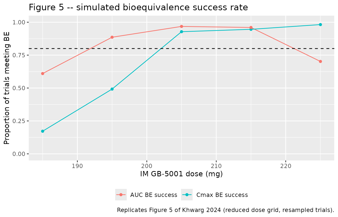
Assumptions and deviations
- Two model files, one fit. Khwarg 2024 fitted both formulations in a single NONMEM run and draws them as one diagram in Figure 2, but estimated CL, V2, Q, V3, the IIV structure and the residual-error model separately for each formulation, so the two arms share no parameters and no subjects (the oral and IM cohorts are disjoint). They are therefore packaged as two independent model files, per the library’s replicate-the-author’s-structure policy. A single file would additionally require switching the residual-error model by formulation, which nlmixr2 cannot express within one endpoint.
-
KA5was recovered from the raw PDF. The text extracted from the source PDF silently dropped theKA5row of Table 2. The value used (0.0134 1/h) is from the published table itself, not inferred. - Residual errors are treated as standard deviations, not variances. Table 2 reports the additive term with linear concentration units (138 and 23.5 pg/mL, not squared units), so both terms are read as SDs. The paper does not state the scale explicitly. Reading the proportional terms as variances instead would imply 37% and 47% residual CVs, which is implausible for an assay with 1.2-4.0% within-run precision.
- Oral bioavailability carries IIV around a fixed typical value. F1 is fixed to 1 with an estimated IIV of 0.0162, exactly as published; individual F1 values can therefore exceed 1. This is the authors’ parameterization, retained as-is.
-
IM
Cmaxsits about 15-20% below the published arithmetic means. Two rows (IM 140 and 280 mg) exceed the 20% flag. The typical-value check above shows this is a level offset, not a structural error:Cmaxper mg is exactly constant across the three doses andTmaxis 434 h at every dose, matching the published median of 432-434 h. Three things account for the offset, and none of them was tuned away. (1) Table 1 reports arithmetic means of N = 9 observed participants per IM arm, whereas the model’s typical-value profile is a median; with 144.8% CV IIV on the IM central volume the two are not the same quantity.- The observed SDs are large (11.72 ug/L at 280 mg), so each published
mean carries roughly 3.9 ug/L of standard error and the typical-value
Cmaxof 40.5 ug/L is within about 1.8 standard errors of the reported 47.63. (3) The parameters reproduce the paper’s Table 2 exactly, andAUCinfmatchesDose / CLto the digit, so the disposition is right; only the peak height of the absorption profile differs, which is where a three-phase absorption model fitted to 9 participants per arm is least well determined.
- The observed SDs are large (11.72 ug/L at 280 mg), so each published
mean carries roughly 3.9 ug/L of standard error and the typical-value
-
Vz/Ffor the IM arms reflects flip-flop kinetics. The paper notes the IM terminal half-life is roughly twice the oral one and that absorption is much slower than elimination, so the NCA-derivedVd/Fis an apparent value driven by the absorption rate rather than true distribution volume. It is reproduced here for completeness, not as a distribution-volume check. -
The oral terminal half-life is sampling-window
dependent. The simulated oral half-life (~63 h) sits below the
published 88 (SD 30) h. Donepezil’s oral profile has a long shallow
terminal phase driven by the 1080 L peripheral compartment, and the
paper’s oral sampling stops at 240 h, so the estimated
lambda.zdepends heavily on which points the terminal-phase regression selects. PKNCA’s automatic window selection and the authors’ manual WinNonlin selection need not agree. With n = 12 and an SD of 30 h the published mean carries roughly 9 h of standard error, so the two are within about 3 standard errors. No parameter was tuned to close this gap. - BE simulation is a reduced replication. The paper swept 9 IM doses (185-225 mg in 5 mg steps) x 10 total sample sizes (50-104 in steps of 6) with 500 freshly simulated trials each. This vignette sweeps 5 IM doses at one total sample size (96) and forms the 500 replicate trials by resampling from a 200-subject simulated pool per arm, to stay inside the vignette render budget. The published per-trial simulation and this resampling scheme agree in expectation but the resampled success rates carry slightly different finite-pool variability.
- The AUC comparison is normalized to a common 28-day window. The paper states only that Cmax and AUC were computed “at steady state” for a once-daily oral regimen against a 4-weekly IM regimen, without spelling out the normalization. Here the oral steady-state daily AUC is multiplied by 28 to match the IM 4-week dosing interval; this is the normalization under which the published AUC-equivalent dose (~195-205 mg) reproduces.
- No covariates. The final model retained none, so the virtual cohorts carry no covariate distributions; between-subject differences come entirely from the published IIV.