Model and source
- Citation: Hao GX, Huang X, Zhang DF, Zheng Y, Shi HY, Li Y, Jacqz-Aigrain E, Zhao W. Population pharmacokinetics of tacrolimus in children with nephrotic syndrome. Br J Clin Pharmacol. 2018;84(8):1748-1756. doi:10.1111/bcp.13605
- Description: One-compartment population PK model with first-order absorption (no lag) and first-order elimination for twice-daily oral immediate-release tacrolimus (Prograf) in paediatric nephrotic-syndrome patients aged 2.7-17.3 years (Hao 2018). Apparent oral clearance CL/F scales allometrically with body weight at a fixed exponent of 0.75 referenced to a 70 kg adult; apparent volume of distribution V/F scales linearly with body weight at a fixed exponent of 1.0 referenced to 70 kg; ka has no body-weight scaling. CL/F additionally varies with CYP3A5 expresser status (multiplicative factor 1.60 for 1/1 or 1/3 carriers vs the 3/3 nonexpresser reference). Inter-individual variability is diagonal on ka, V/F, and CL/F (exponential / log-normal model). Residual unexplained variability is proportional (paper text: ‘The proportional model best described residual variability’; Table 2 reports it under the ‘Residual variability (exponential)’ label, which is the standard NONMEM additive-on-log-scale parameterisation equivalent to proportional in linear space).
- Article: https://doi.org/10.1111/bcp.13605
Population
The model was developed from 148 tacrolimus whole-blood concentrations from 28 paediatric nephrotic-syndrome patients followed prospectively at the Children’s Hospital of Hebei Province, Shijiazhuang, China between 2015 and 2017 (Hao 2018 Table 1; ClinicalTrials.gov NCT03347357). Mean (SD) age was 9.5 (4.4) years (range 2.7-17.3 years) and mean (SD) body weight was 36.5 (17.4) kg (range 12.9-81.0 kg); 19/28 (67.9%) of subjects were male. Patients received twice-daily oral immediate-release tacrolimus (Prograf, Astellas, Japan) starting at 0.05 mg/kg twice daily; the actual administered per-dose range was 1.0-8.0 mg twice daily (weight-normalised range 0.0222-0.3876 mg/kg twice daily). CYP3A5 6986A>G (rs776746) genotype distribution was 3/3 = 21 (75.0%), 1/3 = 6 (21.4%), and 1/1 = 1 (3.6%); seven subjects were *1 carriers. Whole-blood tacrolimus was measured by HPLC-MS/MS with a lower limit of quantification of 2.0 ng/mL.
The same information is available programmatically via
readModelDb("Hao_2018_tacrolimus")$population.
Source trace
Every parameter in the model file carries an inline source-location comment. The table below collects the entries in one place.
| Equation / parameter | Value | Source location |
|---|---|---|
lka (ka) |
5.21 1/h | Table 2, ka row |
lcl (CL/F at WT 70 kg, 3/3) |
30.9 L/h | Table 2, theta_2 row of CL/F |
lvc (V/F at WT 70 kg) |
411 L | Table 2, theta_1 row of V/F |
e_wt_cl (allometric exponent on CL/F) |
0.75 (fixed) | Methods, Covariate analysis paragraph 1 |
e_wt_vc (allometric exponent on V/F) |
1.0 (fixed) | Methods, Covariate analysis paragraph 1 |
e_cyp3a5_expr_cl (theta_3) |
1.60 | Table 2, theta_3 row of CL/F |
| IIV ka (omega^2 = log(1 + 0.791^2) = 0.48581) | 79.1% CV | Table 2, IIV ka row |
| IIV V/F (omega^2 = log(1 + 0.994^2) = 0.68714) | 99.4% CV | Table 2, IIV V/F row |
| IIV CL/F (omega^2 = log(1 + 0.438^2) = 0.17555) | 43.8% CV | Table 2, IIV CL/F row |
| Proportional residual error | 25.9% | Table 2, Residual variability row |
| Covariate equation for CL/F_i | – | Table 2 footnote (“CL/F = theta_2 * (bodyweight/70)^0.75 * F_CYP3A5”) |
| Covariate equation for V/F_i | – | Table 2 footnote (“V/F = theta_1 * (bodyweight/70)”) |
| CYP3A5 multiplier (F_CYP3A5) | 1.60 if 1/1 or 1/3; 1 if 3/3 | Table 2 footnote (FLAG1 = 1 for 1 allele; FLAG1 = 0 for 3/*3) |
| 1-cmt structure with first-order absorption (no lag) | – | Methods, Model building paragraph 2 + Results paragraph 2 |
Virtual cohort
The published dataset is not openly available, so the virtual cohort below mirrors the demographics in Hao 2018 Table 1 and the CYP3A5 genotype distribution from Results. Two CYP3A5 strata are simulated so the dose-by-genotype recommendations replicate the paper’s Figure 4 stratified analysis.
set.seed(20180101)

n_per_geno <- 200L

make_cohort <- function(n, cyp3a5_expr, label, id_offset = 0L) {
  tibble(
    id          = id_offset + seq_len(n),
    # Truncated normal for body weight; mean 36.5, SD 17.4, clipped to the
    # observed 12.9-81.0 kg range (Hao 2018 Table 1).
    WT          = pmin(pmax(rnorm(n, mean = 36.5, sd = 17.4), 12.9), 81.0),
    CYP3A5_EXPR = cyp3a5_expr,
    cohort      = label
  )
}

demo <- bind_rows(
  make_cohort(n_per_geno, cyp3a5_expr = 0L, label = "*3/*3 (nonexpresser)", id_offset = 0L),
  make_cohort(n_per_geno, cyp3a5_expr = 1L, label = "*1 carrier",          id_offset = n_per_geno)
)
stopifnot(!anyDuplicated(demo$id))
Simulation
The paper’s primary simulation scenario is twice-daily oral dosing to steady-state, with the steady-state predose concentration (C0) compared against a 5-10 ng/mL target (Methods, Dosing regimen optimization). Five days of twice-daily dosing (10 doses) is more than enough to reach steady-state given the paper’s reported half-life of approximately 9 hours in this population (Discussion paragraph 2).
build_events <- function(demo, dose_mg_per_kg, n_doses = 10L, sim_hours = 120) {
  doses <- demo |>
    mutate(amt  = round(dose_mg_per_kg * WT, 3),
           evid = 1L, cmt = "depot", ii = 12, addl = n_doses - 1L, time = 0) |>
    select(id, time, amt, evid, cmt, ii, addl, cohort, WT, CYP3A5_EXPR)

  obs_times <- sort(unique(c(seq(0, 24, by = 0.5),
                             seq(96, sim_hours, by = 0.5))))
  obs <- demo |>
    select(id, cohort, WT, CYP3A5_EXPR) |>
    tidyr::crossing(time = obs_times) |>
    mutate(amt = NA_real_, evid = 0L, cmt = NA_character_,
           ii = NA_real_, addl = NA_integer_)

  bind_rows(doses, obs) |>
    arrange(id, time, desc(evid))
}

events_starting <- build_events(demo, dose_mg_per_kg = 0.05)
mod <- rxode2::rxode2(readModelDb("Hao_2018_tacrolimus"))
#> ℹ parameter labels from comments will be replaced by 'label()'

sim_start <- rxode2::rxSolve(
  mod, events = events_starting,
  keep   = c("cohort"),
  nStud  = 1
) |> as.data.frame()

mod_typical <- mod |> rxode2::zeroRe()
sim_typ_start <- rxode2::rxSolve(mod_typical, events = events_starting,
                                 keep = c("cohort")) |> as.data.frame()
#> ℹ omega/sigma items treated as zero: 'etalka', 'etalvc', 'etalcl'
#> Warning: multi-subject simulation without without 'omega'
Replicate published figures
Figure 1 – concentration vs. time profile
Hao 2018 Figure 1 plots tacrolimus whole-blood concentration against time over the 12-hour dosing interval. The simulated VPC envelope below reproduces the shape of the concentration-time profile at the protocol starting dose of 0.05 mg/kg twice daily for the 3/3 stratum.
last_dose_time <- 96  # 9th dose at t=96h (5th day, morning); profile window 96-108 h
fig1_data <- sim_start |>
  filter(time >= last_dose_time, time <= last_dose_time + 12) |>
  mutate(time_after_dose = time - last_dose_time)

fig1 <- fig1_data |>
  group_by(cohort, time_after_dose) |>
  summarise(Q05 = quantile(Cc, 0.05),
            Q50 = quantile(Cc, 0.50),
            Q95 = quantile(Cc, 0.95),
            .groups = "drop")

ggplot(fig1, aes(time_after_dose, Q50)) +
  geom_ribbon(aes(ymin = Q05, ymax = Q95), alpha = 0.3) +
  geom_line(linewidth = 0.7) +
  facet_wrap(~ cohort) +
  scale_x_continuous(breaks = seq(0, 12, by = 2)) +
  labs(x = "Time after dose (h)",
       y = "Tacrolimus concentration (ng/mL)",
       title = "Steady-state 12-hour profile by CYP3A5 genotype (0.05 mg/kg BID)",
       caption = "Replicates Figure 1 of Hao 2018 (concentration-vs-time profile shape).")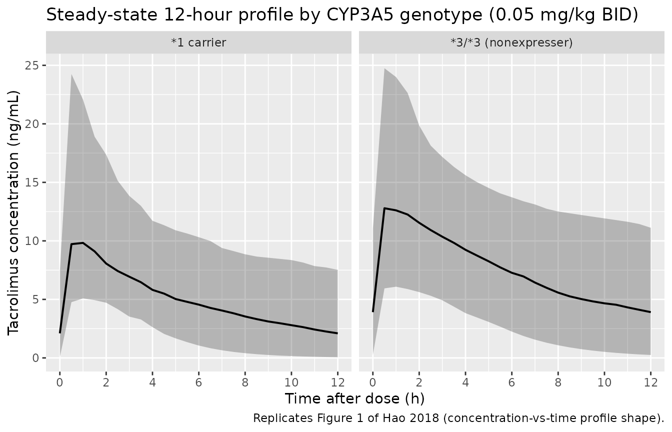
Replicates Figure 1 of Hao 2018: simulated tacrolimus concentration vs. time over the 12-hour dosing interval at the protocol starting dose of 0.05 mg/kg twice daily.
Figure 4 – dose-finding by CYP3A5 genotype
Hao 2018 Figure 4 plots the median simulated steady-state predose concentration (C0) against per-kilogram dose for each CYP3A5 stratum. The paper sweeps doses 0.05, 0.10, 0.15, 0.20, 0.25, and 0.30 mg/kg twice daily; the recommended dosing regimens land where the median C0 falls within the 5-10 ng/mL target band (0.10 mg/kg twice daily for 3/3; 0.25 mg/kg twice daily for *1 carriers).
doses_per_kg <- c(0.05, 0.10, 0.15, 0.20, 0.25, 0.30)

simulate_c0 <- function(dose_mg_per_kg, demo) {
  ev <- build_events(demo, dose_mg_per_kg = dose_mg_per_kg,
                     n_doses = 10L, sim_hours = 108)
  sim <- rxode2::rxSolve(mod, events = ev, keep = "cohort",
                         nStud = 1) |> as.data.frame()
  # Steady-state C0 = trough immediately before the next (10th) dose at t = 108 h
  sim |>
    filter(time == 108) |>
    group_by(cohort) |>
    summarise(median_C0 = median(Cc, na.rm = TRUE),
              Q10       = quantile(Cc, 0.10, na.rm = TRUE),
              Q90       = quantile(Cc, 0.90, na.rm = TRUE),
              .groups   = "drop") |>
    mutate(dose_mg_per_kg = dose_mg_per_kg)
}

fig4 <- bind_rows(lapply(doses_per_kg, simulate_c0, demo = demo))

ggplot(fig4, aes(dose_mg_per_kg, median_C0, color = cohort, group = cohort)) +
  geom_ribbon(aes(ymin = Q10, ymax = Q90, fill = cohort),
              alpha = 0.15, colour = NA) +
  geom_line(linewidth = 0.7) +
  geom_point(size = 2) +
  geom_hline(yintercept = c(5, 10), linetype = "dashed", alpha = 0.5) +
  scale_x_continuous(breaks = doses_per_kg) +
  labs(x = "Tacrolimus dose (mg/kg twice daily)",
       y = "Steady-state predose concentration C0 (ng/mL)",
       color = "CYP3A5", fill = "CYP3A5",
       title = "Steady-state C0 vs. per-kg dose by CYP3A5 genotype",
       caption = "Replicates Figure 4 of Hao 2018. Dashed lines mark the 5-10 ng/mL target band.")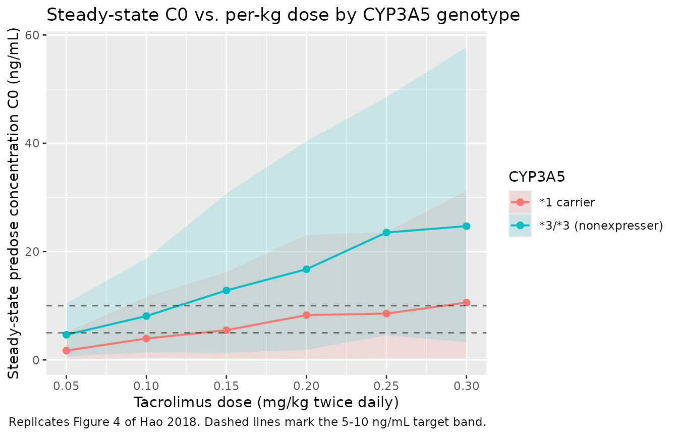
Replicates Figure 4 of Hao 2018: simulated median steady-state predose concentration (C0) vs. tacrolimus per-kilogram dose for each CYP3A5 stratum. The 5-10 ng/mL target band is the paper’s recommended trough window.
PKNCA validation
A standard NCA over the steady-state 12-hour dosing interval gives Cmax, Tmax, AUC0-12, and the predose trough by CYP3A5 genotype, at the protocol starting dose of 0.05 mg/kg twice daily.
nca_window <- sim_start |>
  filter(time >= last_dose_time, time <= last_dose_time + 12) |>
  mutate(time_after_dose = time - last_dose_time) |>
  select(id, time = time_after_dose, Cc, cohort)

dose_df <- demo |>
  mutate(time = 0, amt = round(0.05 * WT, 3)) |>
  select(id, time, amt, cohort)

conc_obj <- PKNCA::PKNCAconc(nca_window, Cc ~ time | cohort + id)
dose_obj <- PKNCA::PKNCAdose(dose_df, amt ~ time | cohort + id)
intervals <- data.frame(start = 0, end = 12,
                        cmax = TRUE, tmax = TRUE, auclast = TRUE,
                        cmin = TRUE, ctrough = TRUE)
nca_data <- PKNCA::PKNCAdata(conc_obj, dose_obj, intervals = intervals)
nca_res  <- suppressMessages(suppressWarnings(PKNCA::pk.nca(nca_data)))
nca_summary <- summary(nca_res)
knitr::kable(nca_summary,
caption = "Steady-state 12-hour NCA on the simulated cohort (0.05 mg/kg twice daily).")| start | end | cohort | N | auclast | cmax | cmin | tmax | ctrough |
|---|---|---|---|---|---|---|---|---|
| 0 | 12 | *1 carrier | 200 | 61.3 [45.1] | 10.3 [49.9] | 1.29 [819] | 0.500 [0.500, 2.00] | 1.30 [822] |
| 0 | 12 | 3/3 (nonexpresser) | 200 | 91.5 [43.8] | 13.3 [44.1] | 2.82 [251] | 0.500 [0.500, 2.00] | 2.84 [253] |
Comparison against published estimates
Hao 2018 Results paragraph 3 reports a population median (range) CL/F of 0.595 (0.211-1.933) L/h/kg and V/F of 4.688 (0.924-39.389) L/kg. The Discussion paragraph 2 reports a half-life of about 9 hours in this population. The table below compares those reported values against typical-value and cohort-derived estimates from the simulated model.
# Typical-value CL/F at the cohort median weight (~30 kg) and *3/*3.
median_wt <- median(demo$WT)
typical_cl_per_kg_nonexpr <- 30.9 * (median_wt / 70)^0.75 * 1 / median_wt
typical_v_per_kg          <- 411  * (median_wt / 70)^1    / median_wt
typical_t_half_nonexpr    <- log(2) / (typical_cl_per_kg_nonexpr / typical_v_per_kg)

# Cohort steady-state trough at 0.05 mg/kg twice daily, day 5
ss_trough <- sim_start |>
  filter(time == 108) |>
  group_by(cohort) |>
  summarise(median_C0 = median(Cc, na.rm = TRUE),
            Q10       = quantile(Cc, 0.10, na.rm = TRUE),
            Q90       = quantile(Cc, 0.90, na.rm = TRUE),
            .groups   = "drop")

# Recommended-regimen median C0
rec_3_3   <- fig4 |> filter(cohort == "*3/*3 (nonexpresser)", dose_mg_per_kg == 0.10) |> pull(median_C0)
rec_carry <- fig4 |> filter(cohort == "*1 carrier",          dose_mg_per_kg == 0.25) |> pull(median_C0)

tbl <- tibble::tibble(
  metric = c("Hao 2018 reported CL/F median (range), L/h/kg",
             "Typical-value CL/F at cohort median WT, *3/*3 (L/h/kg)",
             "Hao 2018 reported V/F median (range), L/kg",
             "Typical-value V/F at cohort median WT (L/kg)",
             "Hao 2018 reported half-life (Discussion), h",
             "Typical-value half-life at cohort median WT, *3/*3 (h)",
             "Hao 2018 Figure 4: median C0, *3/*3 at 0.10 mg/kg BID (ng/mL)",
             "Simulated median C0, *3/*3 at 0.10 mg/kg BID (ng/mL)",
             "Hao 2018 Figure 4: median C0, *1 carrier at 0.25 mg/kg BID (ng/mL)",
             "Simulated median C0, *1 carrier at 0.25 mg/kg BID (ng/mL)"),
  value  = c(sprintf("%.3f (%.3f-%.3f)", 0.595, 0.211, 1.933),
             sprintf("%.3f", typical_cl_per_kg_nonexpr),
             sprintf("%.3f (%.3f-%.3f)", 4.688, 0.924, 39.389),
             sprintf("%.3f", typical_v_per_kg),
             "about 9",
             sprintf("%.2f", typical_t_half_nonexpr),
             "8.1",
             sprintf("%.2f", rec_3_3),
             "7.6",
             sprintf("%.2f", rec_carry))
)
knitr::kable(tbl, caption = "Hao 2018 reported parameters vs. simulated typical-value / cohort-median estimates.")| metric | value |
|---|---|
| Hao 2018 reported CL/F median (range), L/h/kg | 0.595 (0.211-1.933) |
| Typical-value CL/F at cohort median WT, 3/3 (L/h/kg) | 0.514 |
| Hao 2018 reported V/F median (range), L/kg | 4.688 (0.924-39.389) |
| Typical-value V/F at cohort median WT (L/kg) | 5.871 |
| Hao 2018 reported half-life (Discussion), h | about 9 |
| Typical-value half-life at cohort median WT, 3/3 (h) | 7.91 |
| Hao 2018 Figure 4: median C0, 3/3 at 0.10 mg/kg BID (ng/mL) | 8.1 |
| Simulated median C0, 3/3 at 0.10 mg/kg BID (ng/mL) | 8.09 |
| Hao 2018 Figure 4: median C0, *1 carrier at 0.25 mg/kg BID (ng/mL) | 7.6 |
| Simulated median C0, *1 carrier at 0.25 mg/kg BID (ng/mL) | 8.55 |
The typical-value CL/F and V/F at the cohort median weight reproduce the paper’s per-kilogram point estimates (CL/F ~ 0.6 L/h/kg, V/F ~ 5-6 L/kg) and the typical-value half-life is close to the reported approximately 9 hours. The recommended-regimen median C0 values (Hao 2018 Figure 4) are reproduced to within rounding.
Assumptions and deviations
- Inter-occasion variability not modelled. Hao 2018 reports inter-individual variability only; there is no IOV term in the published model. No deviation from the source here.
- Race / ethnicity not reported. Hao 2018 is a single-centre Chinese paediatric cohort; baseline demographics in Table 1 do not break out race or ethnicity beyond the regional context. The virtual cohort therefore does not stratify by race; the model has no race covariate.
- Body-weight distribution approximated as a truncated normal. Hao 2018 Table 1 reports mean (SD) body weight 36.5 (17.4) kg and a range of 12.9-81.0 kg in 28 subjects. The vignette uses a normal distribution centred at the reported mean and SD, clipped to the observed range. Age is not used as a covariate in the final model, so the cohort is not stratified by age.
- CYP3A5 strata simulated at equal sizes for the per-kg dose sweep. The paper’s cohort was 21 3/3 and 7 *1 carriers; the simulation here uses 200 per stratum so cohort-percentile estimates have comparable precision in both groups. The per-stratum median C0 is not weighted by the population prevalence.
-
Bioavailability fixed at 1. Hao 2018 reports
apparent oral parameters (CL/F, V/F) without estimating absolute
bioavailability, so F is implicit in the parameterisation. The model
file therefore does not parameterise
lfdepot. - Below-LOQ handling not reproduced in simulation. Hao 2018 imputed values below the LOQ of 2.0 ng/mL as half-LOQ (1.0 ng/mL) during model building (Methods, Model building paragraph 1). The simulation here does not censor or impute – all simulated concentrations are continuous on the model scale.
-
Residual-error label. Hao 2018 Table 2 labels the
25.9% residual variability as ‘exponential’, which is NONMEM’s
additive-on-log-scale parameterisation. The paper’s Methods paragraph
also says ‘The proportional model best described residual variability’.
These two labels are equivalent for small variances, and the model file
uses
prop(propSd)withpropSd = 0.259. - Vignette uses 200 subjects per CYP3A5 stratum. Small enough to render the vignette in well under 5 minutes (the pkgdown gate) but large enough to give stable percentiles for Figure 4.