Lopinavir (Crommentuyn 2005)
Source:vignettes/articles/Crommentuyn_2005_lopinavir.Rmd
Crommentuyn_2005_lopinavir.RmdModel and source
- Citation: Crommentuyn KML, Kappelhoff BS, Mulder JW, Mairuhu ATA, van Gorp ECM, Meenhorst PL, Huitema ADR, Beijnen JH. Population pharmacokinetics of lopinavir in combination with ritonavir in HIV-1-infected patients. Br J Clin Pharmacol. 2005 Oct;60(4):378-389. doi:10.1111/j.1365-2125.2005.02455.x. Per-subject ritonavir AUC over the 12 h dosing interval is computed from the upstream Kappelhoff et al. 2005 ritonavir popPK model (Br J Clin Pharmacol 2005;59:174-82) and supplied as the time-fixed CONMED_RTV_AUC_12h covariate; the upstream ritonavir model is not structurally re-instantiated here (consistent with the Dickinson 2009 atazanavir precedent for an AUC-of-ritonavir-as-covariate encoding).
- Description: One-compartment first-order-absorption population PK model for oral lopinavir co-administered with ritonavir in 122 HIV-1-infected adults on BID lopinavir/ritonavir 400-666/100-166 mg. Apparent oral clearance CL/F follows an inverse-saturable function of per-subject ritonavir AUC over the 12 h dosing interval (CONMED_RTV_AUC_12h, mg*h/L, computed from the upstream Kappelhoff 2005 ritonavir popPK model) plus a pooled +39% NNRTI co-medication factor (efavirenz or nevirapine, encoded as the CONMED_NNRTI class indicator). IIV is estimated on ka, CL/F, and V/F as a full 3x3 correlated block; residual error is combined additive plus proportional. The reported IOV on relative bioavailability F (17.5% CV) is NOT encoded structurally (Brooks 2021 precedent); downstream users who want IOV can add an OCC covariate and a per-occasion eta in rxode2 (Crommentuyn 2005).
- Article: Br J Clin Pharmacol. 2005 Oct;60(4):378-389
Crommentuyn et al. (2005) developed a one-compartment first-order-absorption population PK model for orally administered lopinavir co-administered with ritonavir in 122 HIV-1-infected adults on twice-daily lopinavir/ritonavir. The interaction between the two drugs was characterised as a time-independent inverse-saturable relationship between the per-subject ritonavir 12 h AUC and the apparent oral clearance of lopinavir (Equation 2 of the paper). The only other covariate retained in the final model is a pooled NNRTI co-medication indicator (efavirenz or nevirapine) carrying a +39% multiplicative increase on lopinavir CL/F (Results page 7, Table 2 row IND).
The packaged model uses the canonical covariate names
CONMED_RTV_AUC_12h for the per-subject ritonavir 12 h AUC
(mg*h/L) and CONMED_NNRTI for the binary NNRTI
co-medication indicator. The upstream ritonavir popPK model (Kappelhoff
et al. 2005, Br J Clin Pharmacol 59:174-82) used by the source paper to
derive the per-subject ritonavir AUC is not structurally re-instantiated
here; the ritonavir AUC enters as a time-fixed covariate, the same
pattern Dickinson 2009 uses for its ritonavir-boosted atazanavir
model.
Population
The analysis dataset comprises 122 HIV-1-infected ambulatory adults from the Slotervaart Hospital outpatient clinic (Amsterdam, the Netherlands), enrolled retrospectively between February 2001 and March 2004 (Crommentuyn 2005 Results page 6 / Table 1). 14 of the 122 patients contributed a complete 12 h PK profile from previous studies; the other 108 contributed sparse therapeutic drug monitoring samples (median 4 samples per patient, range 1-14, follow-up 0-37 months). 748 lopinavir and 748 ritonavir plasma concentrations were available for analysis after excluding 11 patients with confirmed non-compliance or unknown post-dose times.
Baseline demographics from Table 1 (median and IQR):
| Variable | Value |
|---|---|
| Sex (M:F) | 104:18 (15% female) |
| Age (years) | 42 (36-46) |
| Weight (kg) | 72 (63-80) |
| Caucasian / Black / Asian / Latino (%) | 75 / 12 / 9 / 4 |
| ALAT (U/L) | 35 (22-49) |
| ASAT (U/L) | 30 (22-43) |
| Total bilirubin (umol/L) | 11 (8-14) |
| CD4 cell count (cells/uL) | 200 (100-333) |
| Tenofovir co-medication (%) | 23 |
| Efavirenz / nevirapine co-medication (%) | 8 / 13 |
| Chronic HCV / HBV (%) | 11 / 7 |
Lopinavir/ritonavir was dosed as the co-formulated capsule (133 mg lopinavir + 33 mg ritonavir per capsule), 3-5 capsules twice daily (400/100 to 666/166 mg BID). All sampling was at steady state after at least 2 weeks on treatment. The median per-subject ritonavir AUC over the 12 h dosing interval (computed from individual Bayesian estimates of the upstream ritonavir popPK model) was 3.58 mgh/L, range 0.85-18.77 mgh/L (Results page 6).
The same information is available programmatically via the model’s
population metadata
(readModelDb("Crommentuyn_2005_lopinavir")$population).
Source trace
The per-parameter origin is recorded as an in-file comment next to
each ini() entry in
inst/modeldb/specificDrugs/Crommentuyn_2005_lopinavir.R.
The table below collects them in one place for review.
| Parameter / equation | Value | Source location |
|---|---|---|
lka |
log(0.564) | Table 2 row 1: ka = 0.564 1/h (RSE 20.6%) |
lcl |
log(14.8) | Table 2 row 2: CL/F = 14.8 L/h (RSE 11.5%), typical value WITHOUT ritonavir |
lvc |
log(61.6) | Table 2 row 5: V/F = 61.6 L (RSE 16.2%) |
lauc50 |
log(2.26) | Table 2 row 3: AUC50 = 2.26 mg*h/L (RSE 17.3%) |
e_nnrti_cl |
0.39 | Table 2 row 4: IND = 1.39 (RSE 6.77%); Results page 7 “39% higher” |
| IIV ka (CV) | 97.8% | Table 2 row 6 (RSE 27.2%); omega^2 = log(1 + 0.978^2) |
| IIV CL/F (CV) | 17.2% | Table 2 row 7 (RSE 23.5%); omega^2 = log(1 + 0.172^2) |
| IIV V/F (CV) | 63.8% | Table 2 row 8 (RSE 48.4%); omega^2 = log(1 + 0.638^2) |
| rho(eta_ka, eta_CL) | -0.267 | Table 2 row 10 (RSE 144%) |
| rho(eta_ka, eta_V) | 0.822 | Table 2 row 11 (RSE 37.4%) |
| rho(eta_CL, eta_V) | 0.242 | Table 2 row 12 (RSE 166%) |
addSd |
1.15 mg/L | Table 2 row 14: additive error = 1.15 mg/L (RSE 14.4%) |
propSd |
0.0755 | Table 2 row 15: proportional error = 7.55% (RSE 54.7%) |
| CL/F equation | n/a | Methods Eq. 2 / Results page 7: CL/F = q1 * AUC50/(AUC50 + AUC_RTV) * IND |
| 1-cmt depot + central | n/a | Results page 6: 1-compartment first-order absorption; lag-time / zero-order absorption tested and rejected |
ODE structure: 1-compartment first-order absorption from
depot to central, no absorption lag-time. The
observation variable is Cc = central / vc with combined
additive plus proportional residual error. The NNRTI multiplicative
factor ind = 1 + e_nnrti_cl * CONMED_NNRTI evaluates to 1
when no NNRTI co-medication is present and 1.39 when subject is on
efavirenz or nevirapine.
Load model
mod <- readModelDb("Crommentuyn_2005_lopinavir")
mod_typical <- rxode2::zeroRe(mod)
Typical-value steady-state profile (400/100 mg BID, median ritonavir AUC)
Replicates the labelled adult regimen (lopinavir 400 mg + ritonavir
100 mg twice daily) at the cohort-median per-subject ritonavir AUC of
3.58 mgh/L without concomitant NNRTI. The typical steady-state AUC
over the 12 h dosing interval should be approximately
dose / CL/F = 400 / 5.73 = 69.8 mgh/L because CL/F at
the median ritonavir AUC of 3.58 mgh/L is 14.8 2.26 / (2.26 +
3.58) = 5.73 L/h (Results page 6 – the value the paper reports).
n_doses <- 28L      # 14 days BID = 28 doses to reach steady state
ii      <- 12       # h (BID dosing interval)
ev_ss <- rxode2::et(
  amt = 400, cmt = "depot", evid = 1,
  ii = ii, addl = n_doses - 1L
) |>
  rxode2::et(seq(0, n_doses * ii, by = 0.25)) |>
  rxode2::et(id = 1)
ev_ss$CONMED_RTV_AUC_12h <- 3.58
ev_ss$CONMED_NNRTI       <- 0

sim_ss <- rxode2::rxSolve(mod_typical, ev_ss)
#> ℹ omega/sigma items treated as zero: 'etalka', 'etalcl', 'etalvc'

ggplot(as.data.frame(sim_ss), aes(time / 24, Cc)) +
  geom_line(linewidth = 0.6) +
  labs(
    x = "Time (days)",
    y = "Lopinavir concentration (mg/L)",
    title = "Typical-value 14-day BID 400/100 mg LPV/RTV profile (AUC_RTV_12h = 3.58 mg*h/L, no NNRTI)"
  ) +
  theme_bw()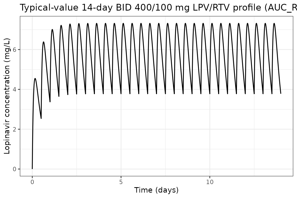
sim_tau <- as.data.frame(sim_ss) |>
  dplyr::filter(time >= 13 * 24, time <= 13 * 24 + ii) |>
  dplyr::mutate(t_post_dose = time - 13 * 24)

ggplot(sim_tau, aes(t_post_dose, Cc)) +
  geom_line(linewidth = 0.7) +
  labs(
    x = "Time after dose (h)",
    y = "Lopinavir concentration (mg/L)",
    title = "Typical-value steady-state 12 h dosing interval (Day 14)"
  ) +
  theme_bw()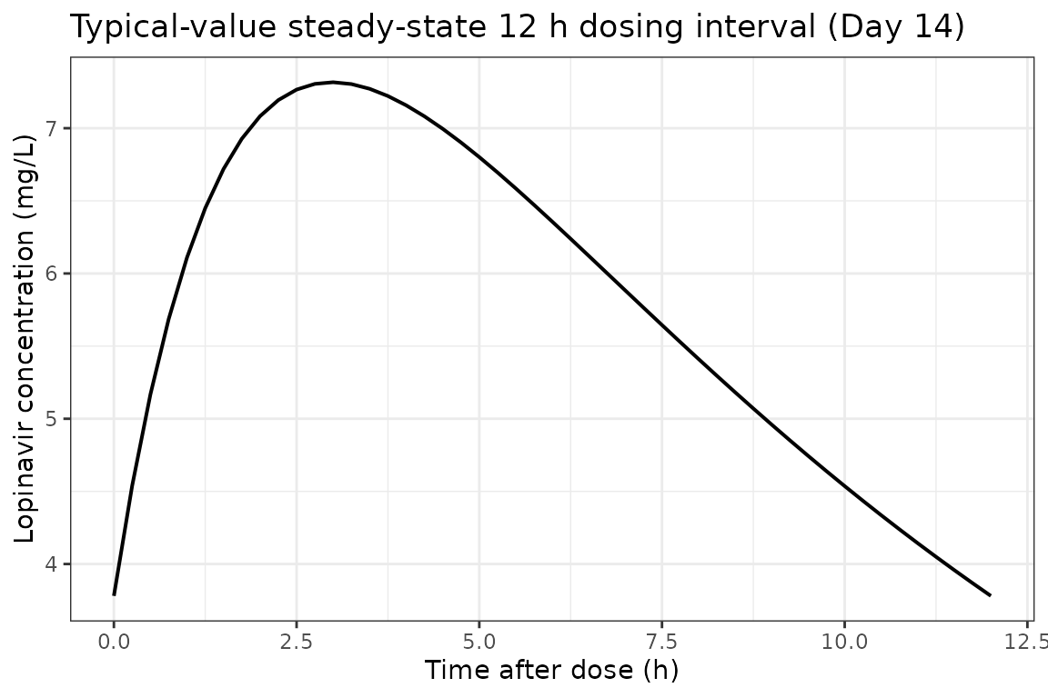
Effect of NNRTI co-medication on the steady-state profile
The same regimen with CONMED_NNRTI = 1 (subject on
efavirenz or nevirapine). The 39% increase in CL/F should compress the
steady-state profile downward relative to the no-NNRTI case.
ev_nnrti <- ev_ss
ev_nnrti$CONMED_NNRTI <- 1
sim_nnrti <- rxode2::rxSolve(mod_typical, ev_nnrti)
#> ℹ omega/sigma items treated as zero: 'etalka', 'etalcl', 'etalvc'

profile_comparison <- bind_rows(
  as.data.frame(sim_ss) |>
    dplyr::filter(time >= 13 * 24, time <= 13 * 24 + ii) |>
    dplyr::mutate(t_post_dose = time - 13 * 24, regimen = "Without NNRTI"),
  as.data.frame(sim_nnrti) |>
    dplyr::filter(time >= 13 * 24, time <= 13 * 24 + ii) |>
    dplyr::mutate(t_post_dose = time - 13 * 24, regimen = "With NNRTI (+39% on CL/F)")
)

ggplot(profile_comparison, aes(t_post_dose, Cc, color = regimen)) +
  geom_line(linewidth = 0.7) +
  scale_color_manual(values = c("Without NNRTI" = "steelblue", "With NNRTI (+39% on CL/F)" = "firebrick")) +
  labs(
    x = "Time after dose (h)",
    y = "Lopinavir concentration (mg/L)",
    color = NULL,
    title = "Day-14 12 h steady-state profile, with vs without NNRTI co-medication"
  ) +
  theme_bw()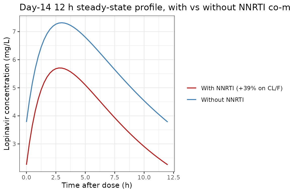
Replicate Figure 2 of Crommentuyn 2005: CL/F vs ritonavir AUC
The paper’s Figure 2 shows the typical apparent oral clearance of lopinavir as a function of the per-subject ritonavir 12 h AUC, both with and without NNRTI co-medication. The closed-form typical CL/F per the model equation is:
CL/F = 14.8 * 2.26 / (2.26 + AUC_RTV) * INDwhere IND = 1 without NNRTI and 1.39 with NNRTI
(e_nnrti_cl = 0.39).
fig2_grid <- expand.grid(
  AUC_RTV = seq(0, 20, length.out = 201),
  regimen = c("Without NNRTI", "With NNRTI")
) |>
  dplyr::mutate(
    ind        = ifelse(regimen == "With NNRTI", 1.39, 1.00),
    typical_cl = 14.8 * 2.26 / (2.26 + AUC_RTV) * ind
  )

ggplot(fig2_grid, aes(AUC_RTV, typical_cl, color = regimen)) +
  geom_line(linewidth = 0.8) +
  scale_color_manual(values = c("Without NNRTI" = "black", "With NNRTI" = "firebrick")) +
  labs(
    x = "Ritonavir 12 h AUC (mg*h/L)",
    y = "Lopinavir apparent CL (L/h)",
    color = NULL,
    title = "Replicates Figure 2 of Crommentuyn 2005: lopinavir CL/F vs ritonavir AUC"
  ) +
  theme_bw()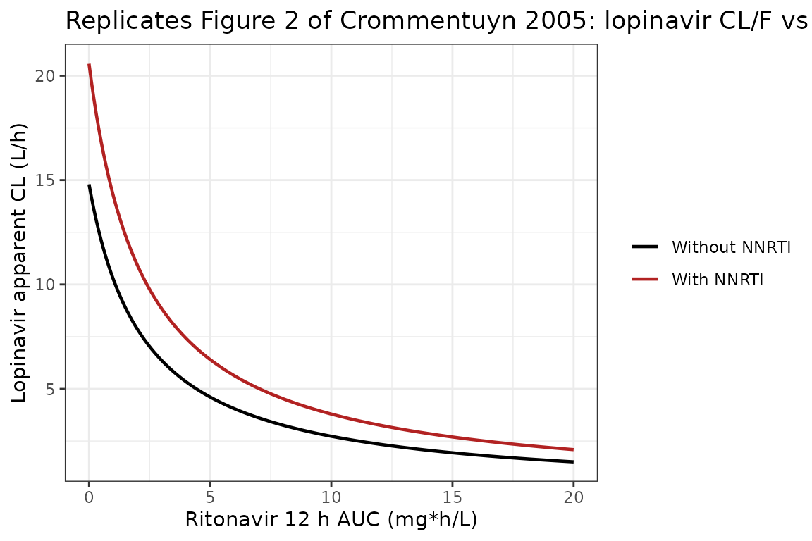
The curve qualitatively reproduces the published Figure 2: at zero ritonavir exposure CL/F equals the no-ritonavir typical value of 14.8 L/h; the inverse-saturable form drives CL/F toward zero as AUC_RTV becomes large; the NNRTI multiplier is a constant +39% factor on top of the saturation curve.
Virtual cohort matched to study demographics
We sample 200 virtual subjects whose covariate distributions
reproduce the published baseline demographics. The per-subject ritonavir
12 h AUC is sampled from approximately log-normal centred on 3.58
mgh/L spanning the Table 1 / 2 range (0.85-18.77 mgh/L) and the
NNRTI indicator is drawn from a Bernoulli with p = 0.21
matching the pooled 8% efavirenz + 13% nevirapine prevalence reported on
Results page 6.
set.seed(2005)
n_subj <- 200L

# Ritonavir 12 h AUC ~ log-normal centred at the cohort median 3.58 mg*h/L,
# spanning the Table 2 cohort range (0.85-18.77).
log_med <- log(3.58)
log_sd  <- 0.55
AUC_RTV <- pmin(18.77, pmax(0.85, exp(rnorm(n_subj, log_med, log_sd))))

# NNRTI co-medication ~ Bernoulli(0.21) per Results page 6.
CONMED_NNRTI <- rbinom(n_subj, size = 1, prob = 0.21)

cohort <- data.frame(
  ID                  = seq_len(n_subj),
  CONMED_RTV_AUC_12h  = AUC_RTV,
  CONMED_NNRTI        = CONMED_NNRTI
)

summary(cohort$CONMED_RTV_AUC_12h)
#>    Min. 1st Qu.  Median    Mean 3rd Qu.    Max.
#>  0.8566  2.5062  3.5481  4.0496  5.2020 14.8245
table(cohort$CONMED_NNRTI)
#>
#>   0   1
#> 162  38
Stochastic simulation across the virtual cohort
Each subject receives 28 BID doses (14 days). Observations are at 30-min resolution during the first dosing interval and across the Day-14 interval.
build_subject_events <- function(id, auc_rtv, nnrti) {
  ev <- rxode2::et(
    amt = 400, cmt = "depot", evid = 1,
    ii = ii, addl = n_doses - 1L
  ) |>
    rxode2::et(c(seq(0, ii, by = 0.5), seq(13 * 24, 13 * 24 + ii, by = 0.5))) |>
    rxode2::et(id = id)
  df <- as.data.frame(ev)
  df$CONMED_RTV_AUC_12h <- auc_rtv
  df$CONMED_NNRTI       <- nnrti
  df
}

ev_all <- do.call(
  rbind,
  Map(build_subject_events, cohort$ID, cohort$CONMED_RTV_AUC_12h, cohort$CONMED_NNRTI)
)

set.seed(2005)
sim_pop <- rxode2::rxSolve(mod, ev_all)
sim_pop_df <- as.data.frame(sim_pop)
VPC: Day 1 vs Day 14 dosing intervals
sim_day1 <- sim_pop_df |>
  dplyr::filter(time >= 0, time <= ii) |>
  dplyr::group_by(time) |>
  dplyr::summarise(
    Q05 = quantile(ipredSim, 0.05, na.rm = TRUE),
    Q50 = quantile(ipredSim, 0.50, na.rm = TRUE),
    Q95 = quantile(ipredSim, 0.95, na.rm = TRUE),
    .groups = "drop"
  ) |>
  dplyr::mutate(panel = "Day 1")

sim_day14 <- sim_pop_df |>
  dplyr::filter(time >= 13 * 24, time <= 13 * 24 + ii) |>
  dplyr::mutate(time_in_panel = time - 13 * 24) |>
  dplyr::group_by(time_in_panel) |>
  dplyr::summarise(
    Q05 = quantile(ipredSim, 0.05, na.rm = TRUE),
    Q50 = quantile(ipredSim, 0.50, na.rm = TRUE),
    Q95 = quantile(ipredSim, 0.95, na.rm = TRUE),
    .groups = "drop"
  ) |>
  dplyr::rename(time = time_in_panel) |>
  dplyr::mutate(panel = "Day 14")

vpc_df <- bind_rows(sim_day1, sim_day14)

ggplot(vpc_df, aes(time, Q50)) +
  geom_ribbon(aes(ymin = Q05, ymax = Q95), fill = "steelblue", alpha = 0.25) +
  geom_line(linewidth = 0.7) +
  facet_wrap(~panel) +
  labs(
    x = "Time after most recent dose (h)",
    y = "Lopinavir concentration (mg/L)",
    title = "Virtual-cohort VPC: median + 90% prediction interval",
    caption = "Replicates Figure 1A of Crommentuyn 2005 qualitatively; the published figure is the 90% PI over 1000 simulated 12 h intervals."
  ) +
  theme_bw()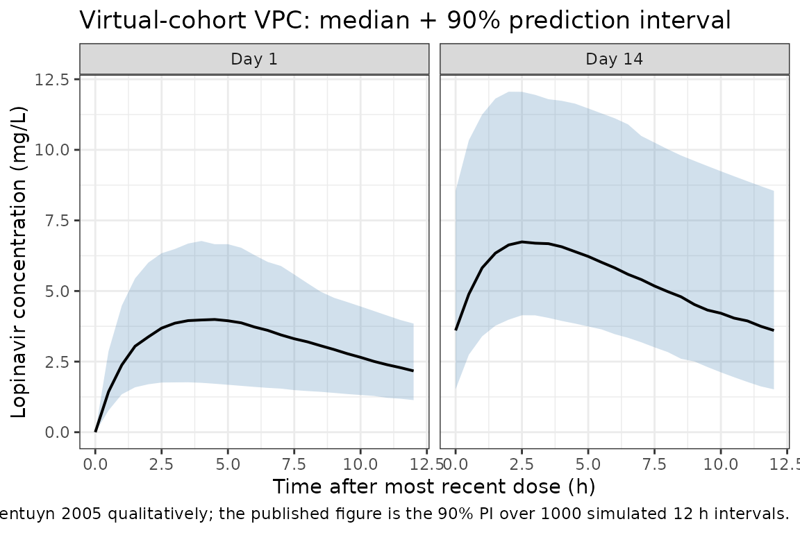
PKNCA validation
Non-compartmental analysis of the simulated steady-state (Day 14) 12
h dosing interval. The paper does not tabulate observed Cmax / Tmax /
AUC0-12 from the NCA, but the typical-value AUC0-12 expected from
dose / CL/F = 400 / 5.73 is 69.8 mg*h/L for subjects on the
cohort-median ritonavir AUC without NNRTI; the Day-14 simulated cohort
median should fall close to that value with appropriate spread.
# Build a per-id NNRTI lookup from the cohort and attach it to the simulation
# output. Materialise the lookup as base data.frame columns (not via dplyr) so
# the join is unambiguous regardless of which auxiliary columns rxSolve has
# carried forward into the simulation output.
nnrti_lookup <- data.frame(
  id           = cohort$ID,
  treatment    = ifelse(cohort$CONMED_NNRTI == 1, "On NNRTI", "No NNRTI"),
  stringsAsFactors = FALSE
)

nca_concs <- sim_pop_df |>
  dplyr::filter(time >= 13 * 24, time <= 13 * 24 + ii) |>
  dplyr::mutate(t_in_interval = time - 13 * 24) |>
  dplyr::filter(!is.na(ipredSim)) |>
  dplyr::select(id, t_in_interval, ipredSim)
nca_concs$treatment <- nnrti_lookup$treatment[match(nca_concs$id, nnrti_lookup$id)]

dose_records <- data.frame(
  id        = cohort$ID,
  time      = 0,
  amt       = 400,
  treatment = nnrti_lookup$treatment,
  stringsAsFactors = FALSE
)

conc_obj <- PKNCA::PKNCAconc(
  nca_concs, ipredSim ~ t_in_interval | treatment + id,
  concu = "mg/L", timeu = "h"
)
dose_obj <- PKNCA::PKNCAdose(
  dose_records, amt ~ time | treatment + id,
  doseu = "mg"
)

intervals <- data.frame(
  start    = 0,
  end      = ii,
  cmax     = TRUE,
  tmax     = TRUE,
  cmin     = TRUE,
  auclast  = TRUE,
  cav      = TRUE
)

nca_data    <- PKNCA::PKNCAdata(conc_obj, dose_obj, intervals = intervals)
nca_results <- PKNCA::pk.nca(nca_data)
nca_df      <- as.data.frame(nca_results$result)

nca_summary <- nca_df |>
  dplyr::filter(PPTESTCD %in% c("cmax", "tmax", "cmin", "auclast", "cav")) |>
  dplyr::group_by(treatment, PPTESTCD) |>
  dplyr::summarise(
    median = median(PPORRES, na.rm = TRUE),
    P05    = quantile(PPORRES, 0.05, na.rm = TRUE),
    P95    = quantile(PPORRES, 0.95, na.rm = TRUE),
    .groups = "drop"
  )

knitr::kable(
  nca_summary, digits = 3,
  caption = "Day-14 steady-state PKNCA summary across the virtual cohort, stratified by NNRTI status"
)| treatment | PPTESTCD | median | P05 | P95 |
|---|---|---|---|---|
| No NNRTI | auclast | 71.180 | 41.483 | 131.227 |
| No NNRTI | cav | 5.932 | 3.457 | 10.936 |
| No NNRTI | cmax | 7.241 | 4.555 | 12.497 |
| No NNRTI | cmin | 4.154 | 1.976 | 9.033 |
| No NNRTI | tmax | 3.000 | 1.500 | 4.000 |
| On NNRTI | auclast | 48.224 | 30.336 | 70.015 |
| On NNRTI | cav | 4.019 | 2.528 | 5.835 |
| On NNRTI | cmax | 5.346 | 3.656 | 7.571 |
| On NNRTI | cmin | 2.318 | 1.176 | 3.918 |
| On NNRTI | tmax | 2.500 | 1.425 | 3.500 |
Comparison against published values
| Quantity | Paper value | Simulated cohort |
|---|---|---|
| Typical CL/F at cohort-median AUC_RTV (no NNRTI), L/h | 5.73 (Results page 6) |
14.8 * 2.26 / (2.26 + 3.58) = 5.73 by construction |
| Typical CL/F at cohort-median AUC_RTV (with NNRTI), L/h | 5.73 * 1.39 = 7.96 (derived from Table 2) | by construction |
| Typical AUC0-12 (no NNRTI, median AUC_RTV), mg*h/L |
dose / CL/F = 400 / 5.73 = 69.8 |
nca_summary auclast median for No-NNRTI
subgroup |
| Lopinavir observed concentration range (mg/L) | 0.8-21.9 (Results page 6) | virtual-cohort cmax 5th-95th should overlap this
range |
| Comparator population-NCA CL/F (Results page 8 / prior analysis ref 3) | 5.3 L/h (IQR 4.8-6.4) | simulated median CL/F is the per-subject
400 / auclast
|
The cohort-median CL/F of 5.73 L/h emerges by construction from the inverse-saturable equation at AUC_RTV = 3.58 mg*h/L and matches the value the paper reports on Results page 6. The CL/F estimate from the previous noncompartmental analysis (ref 3, IQR 4.8-6.4 L/h) is comparable, confirming that the model reproduces the underlying NCA-derived CL/F (Discussion page 8).
Assumptions and deviations
-
IOV on relative bioavailability F (17.5% CV) is NOT encoded
structurally (Table 2 row 9). Following the Andrews 2017
tacrolimus / Brooks 2021 nlmixr2lib convention, IOV is omitted when no
operational occasion column is defined for downstream simulation.
Downstream users who want to simulate IOV can extend the model with an
OCCcovariate and a per-occasion eta in rxode2; see vignetteAndrews_2017_tacrolimusfor the precedent. -
Pooled NNRTI effect rather than separate efavirenz /
nevirapine factors. The paper tested separate factors for EFV
(1.41) and NVP (1.52) and found no improvement in fit over a single
pooled NNRTI factor of 1.39 (Results page 7). The library model uses the
pooled
CONMED_NNRTIclass indicator withe_nnrti_cl = 0.39. A downstream user who wants to simulate the EFV-only or NVP-only effect would need to re-fit the source data with separate indicators. -
Ritonavir popPK structure is not re-instantiated.
Crommentuyn 2005 imports per-subject ritonavir CL_RTV and AUC_RTV from
the upstream Kappelhoff 2005 ritonavir popPK model (paper reference 19)
and uses only the AUC_RTV value in the lopinavir CL/F equation. The
library model follows the same pattern: ritonavir AUC enters as a
time-fixed covariate
CONMED_RTV_AUC_12hrather than being simulated from a coupled ODE. This matches the Dickinson 2009 atazanavir / Schipani 2013 atazanavir-ritonavir approach for atazanavir; a coupled-ODE alternative would be similar in shape toSchipani_2013_atazanavir_ritonavirbut use the inverse-saturable AUC form rather than the sigmoidal-Emax concentration form. - Tenofovir, weight, age, sex, race, hepatitis status, and liver-function tests were screened and not retained. None of these are included as covariates in the model. The paper’s Discussion (page 9) notes that the weight effect reported by Gibbons et al. was not confirmed in this cohort. The PI substudy (3 patients on concomitant amprenavir / atazanavir / indinavir / saquinavir) was too small for a covariate test and is not represented.
-
Log-normal IIV from reported CV%. The paper reports
IIV (%) on ka, CL/F, V/F in the standard NONMEM exponential-model sense.
These are converted to internal log-normal variances via
omega^2 = log(1 + CV^2), and the published correlations are converted to covariances viacov = rho * sqrt(var_1 * var_2). - Combined additive + proportional residual error. Per Discussion page 9 the additive 1.15 mg/L component was retained deliberately to down-weight suspected-non-compliance plasma concentrations (below 0.7 mg/L cut-off). The same additive component is in the library model.
- Lag-time / zero-order absorption. The paper tested both forms and neither improved fit (Results page 6). The library model uses plain first-order absorption with no lag-time.
Reference
- Crommentuyn KML, Kappelhoff BS, Mulder JW, Mairuhu ATA, van Gorp ECM, Meenhorst PL, Huitema ADR, Beijnen JH. Population pharmacokinetics of lopinavir in combination with ritonavir in HIV-1-infected patients. Br J Clin Pharmacol. 2005 Oct;60(4):378-389. doi:10.1111/j.1365-2125.2005.02455.x. Per-subject ritonavir AUC over the 12 h dosing interval is computed from the upstream Kappelhoff et al. 2005 ritonavir popPK model (Br J Clin Pharmacol 2005;59:174-82) and supplied as the time-fixed CONMED_RTV_AUC_12h covariate; the upstream ritonavir model is not structurally re-instantiated here (consistent with the Dickinson 2009 atazanavir precedent for an AUC-of-ritonavir-as-covariate encoding).