Polymyxin B (Liang 2023)
Source:vignettes/articles/Liang_2023_polymyxinB.Rmd
Liang_2023_polymyxinB.RmdModel and source
- Citation: Liang D, Liang Z, Deng G, Cen A, Luo D, Zhang C, Ni S. Population pharmacokinetic analysis and dosing optimization of polymyxin B in critically ill patients. Front Pharmacol. 2023;14:1122310. doi:10.3389/fphar.2023.1122310. PMCID PMC10090446.
- Description: Two-compartment intravenous population PK model for polymyxin B in critically ill adults not receiving CRRT or ECMO (Liang 2023). Fitted by nonparametric adaptive grid (NPAG) in Pmetrics. Serum albumin is a power covariate on CL and age is a power covariate on Vc, both normalized to the cohort median (ALB 31.45 g/L, age 68 years) with exponents fixed at -0.95 and +0.95 respectively. Combined additive plus proportional residual error derived from the Pmetrics assay-error polynomial scaled by the final gamma.
- Article: https://doi.org/10.3389/fphar.2023.1122310
- PubMed Central: https://www.ncbi.nlm.nih.gov/pmc/articles/PMC10090446/
Liang et al. fitted a two-compartment intravenous model to steady-state polymyxin B concentrations from critically ill adults using the nonparametric adaptive grid (NPAG) algorithm in Pmetrics 1.9.7. Serum albumin was retained as a power covariate on clearance and age as a power covariate on the central volume of distribution; the resulting model (Table 2, “model 6”) was then used in Monte Carlo simulations to recommend a dosing regimen.
Population
Twenty-two critically ill adults (age 18 years or older) treated with intravenous polymyxin B at a single center in Guangzhou, China between November 2021 and September 2022 contributed 64 plasma concentrations (Table 1, Results 3.1). The cohort was 77.3% male, with median age 68 years (range 31-94), median weight 60 kg (range 50-80), median APACHE-II score 21.5 points (range 15-46), median baseline serum creatinine 75 umol/L (range 33-125), median baseline Cockcroft-Gault creatinine clearance 68.29 mL/min (range 34.05-192.59), and median baseline serum albumin 31.45 g/L (range 23.1-41.5).
Half the cohort had pulmonary infection alone and a further 45.5% had pulmonary infection with sepsis or septicemia; Acinetobacter baumannii was the most common pathogen (50.0%). Patients receiving continuous renal replacement therapy (n = 10) or extracorporeal membrane oxygenation (n = 2) at the time of blood collection were excluded, so the model must not be extrapolated to those settings (Discussion, study limitations).
Dosing was a loading dose of 100-150 mg followed by a maintenance dose of 50-75 mg q12h, infused over 1-2 h. Sampling began at least 48 h after the start of treatment: 24 trough samples, 23 peak samples, and 17 samples 6-8 h after the end of infusion. Total (not unbound) polymyxin B was measured as the sum of polymyxin B1, B2, and B1-Ile by LC-MS/MS.
The same information is available programmatically via the model’s
population metadata:
str(readModelDb("Liang_2023_polymyxinB")()$population)
#> List of 16
#>  $ species       : chr "human"
#>  $ n_subjects    : num 22
#>  $ n_studies     : num 1
#>  $ n_observations: num 64
#>  $ age_range     : chr "31-94 years"
#>  $ age_median    : chr "68 years"
#>  $ weight_range  : chr "50-80 kg"
#>  $ weight_median : chr "60 kg"
#>  $ sex_female_pct: num 22.7
#>  $ disease_state : chr "critically ill adults (>= 18 years) with multidrug-resistant gram-negative bacterial infection; 50.0% pulmonary"| __truncated__
#>  $ renal_function: chr "baseline serum creatinine median 75 umol/L (33-125); baseline Cockcroft-Gault creatinine clearance median 68.29"| __truncated__
#>  $ albumin       : chr "baseline serum albumin median 31.45 g/L (23.1-41.5)"
#>  $ severity      : chr "APACHE-II score median 21.5 points (15-46)"
#>  $ dose_range    : chr "intravenous infusion over 1-2 h; loading dose 100-150 mg, maintenance dose 50-75 mg q12h"
#>  $ regions       : chr "China (single center, Guangzhou)"
#>  $ notes         : chr "Baseline demographics from Table 1. Patients receiving continuous renal replacement therapy (n = 10) or extraco"| __truncated__
Source trace
The per-parameter origin is recorded as an in-file comment next to
each ini() entry in
inst/modeldb/specificDrugs/Liang_2023_polymyxinB.R. The
table below collects them in one place for review.
| Equation / parameter | Value | Source location |
|---|---|---|
d/dt(central) |
n/a | Equation 1:
dX1/dt = RateIV + (Q/Vp)*X2 - (CL/Vc + Q/Vc)*X1
|
d/dt(peripheral1) |
n/a | Equation 2: dX2/dt = (Q/Vc)*X1 - (Q/Vp)*X2
|
lcl |
log(1.22) |
Table 3, CL median (mean 1.24, SD 0.38 L/h) |
lvc |
log(13.52) |
Table 3, Vc median (mean 16.64, SD 12.74 L) |
lq |
log(2.34) |
Table 3, Q median (mean 3.04, SD 2.27 L/h) |
lvp |
log(76.53) |
Table 3, Vp median (mean 66.20, SD 36.25 L) |
e_alb_cl |
fixed(-0.95) |
Table 2, model 6: CL0*(ALB/31.45)^(-0.95)
|
e_age_vc |
fixed(0.95) |
Table 2, model 6: V0*(age/68)^0.95
|
| ALB reference 31.45 g/L | n/a | Table 1, median baseline ALB |
| AGE reference 68 years | n/a | Table 1, median age |
etalcl |
0.088837 |
Table 3, CL between-subject variability 30.48 %CV |
etalvc |
0.461209 |
Table 3, Vc between-subject variability 76.55 %CV |
etalq |
0.444176 |
Table 3, Q between-subject variability 74.78 %CV |
etalvp |
0.262261 |
Table 3, Vp between-subject variability 54.76 %CV |
addSd |
fixed(0.072) |
Methods 2.4 (C0 = 0.1) x Results 3.2 (final gamma
0.72) |
propSd |
fixed(0.108) |
Methods 2.4 (C1 = 0.15) x Results 3.2 (final gamma
0.72) |
Two transcription steps deserve comment.
Between-subject variability. Pmetrics NPAG returns a
discrete nonparametric joint distribution rather than a parametric
OMEGA. Table 3 summarises it by mean, median, SD, and “%CV”, and the %CV
column is exactly SD / mean for all four parameters (for
example CL: 0.38 / 1.24 = 30.6%). Encoding this in nlmixr2
requires a parametric approximation; a log-normal is used, with the
Table 3 median mapped onto
exp(l<param>) (the log-normal median) and the
variance obtained from omega^2 = log(CV^2 + 1).
Residual error. Pmetrics weights each observation by
the reciprocal of SD x gamma, where
SD = C0 + C1*Cobs + C2*Cobs^2 + C3*Cobs^3 with
C0 = 0.1, C1 = 0.15, C2 = C3 = 0
(Methods 2.4) and the final-cycle gamma was 0.72 (Results
3.2). The total residual standard deviation is therefore
0.72 * (0.1 + 0.15*C) = 0.072 + 0.108*C mg/L, which is a
combined additive plus proportional error.
What drives exposure in this model
Before simulating, it is worth writing down what the final model implies. At steady state, the area under the concentration-time curve over 24 h is fixed by clearance alone:
Age enters the model only through Vc, and
Vc does not appear in this expression. Under the
published model, age changes the shape of the concentration-time curve
(peak and trough) but cannot change AUC, and therefore cannot change any
AUC-based probability of target attainment. This is consistent
with the source’s own Figure 3, in which the three panels of each row
(same albumin stratum, ages 34 / 68 / 93) are visually
indistinguishable, but it is not consistent with the paper’s
Conclusion that “the possibility of obtaining an AUC/MIC >= 50
decreased with older age”. See the Assumptions and deviations
section.
The age-invariance is checked explicitly below.
Virtual cohort
Original observed data are not publicly available. The cohorts below are virtual populations whose covariate distributions follow the three albumin strata and the five dosing regimens defined in Methods 2.5.
set.seed(20230329)

n_per_arm <- 100L

alb_strata <- tibble::tribble(
  ~alb_group,        ~alb_lo, ~alb_hi,
  "Ultra-low ALB",      23.1,    24.9,
  "Low ALB",            25.0,    34.9,
  "Normal ALB",         35.0,    41.5
)

regimens <- tibble::tibble(
  regimen    = c("100 mg q12h", "75 mg q12h", "60 mg q12h",
                 "50 mg q12h", "40 mg q12h"),
  dose_mg    = c(100, 75, 60, 50, 40)
) |>
  mutate(daily_mg = dose_mg * 2)

arms <- tidyr::crossing(alb_strata, regimens) |>
  mutate(arm = paste(alb_group, regimen, sep = " | "))

# 30 days of q12h dosing takes the model well past steady state (terminal
# half-life is about 71 h at the typical parameter values), so the final 24 h
# window is a true steady-state interval.
n_doses  <- 60L
tau      <- 12
obs_from <- (n_doses - 2L) * tau   # start of the final 24 h window
obs_to   <- obs_from + 24

# `n` subjects with consecutive IDs starting at `id_offset + 1`. IDs must be
# consecutive across the whole event table: rxSolve re-indexes non-consecutive
# IDs in its output, which silently breaks the id-based join PKNCA makes
# between the concentration and dose objects.
make_arm <- function(n, dose_mg, alb_lo, alb_hi, arm, alb_group, regimen,
                     daily_mg, id_offset = 0L, age = 68) {
  subj <- tibble::tibble(
    id        = id_offset + seq_len(n),
    ALB       = stats::runif(n, alb_lo, alb_hi),
    AGE       = age,
    arm       = arm,
    alb_group = alb_group,
    regimen   = regimen,
    daily_mg  = daily_mg
  )

  doses <- subj |>
    mutate(
      time = 0, amt = dose_mg, evid = 1L, dur = 1,
      ii = tau, addl = n_doses - 1L, cmt = "central"
    )

  obs <- subj |>
    tidyr::crossing(time = seq(obs_from, obs_to, by = 0.25)) |>
    mutate(
      amt = NA_real_, evid = 0L, dur = NA_real_,
      ii = NA_real_, addl = NA_integer_, cmt = "central"
    )

  bind_rows(doses, obs) |> arrange(id, time, desc(evid))
}

events <- do.call(
  bind_rows,
  lapply(seq_len(nrow(arms)), function(i) {
    a <- arms[i, ]
    make_arm(
      n         = n_per_arm,
      dose_mg   = a$dose_mg,
      alb_lo    = a$alb_lo,
      alb_hi    = a$alb_hi,
      arm       = a$arm,
      alb_group = a$alb_group,
      regimen   = a$regimen,
      daily_mg  = a$daily_mg,
      id_offset = (i - 1L) * n_per_arm
    )
  })
)

# Disjoint IDs across arms are mandatory; duplicate IDs silently merge subjects.
stopifnot(!anyDuplicated(unique(events[, c("id", "time", "evid")])))

# ... and they must also be consecutive from 1. rxSolve re-indexes
# non-consecutive IDs in its output, which leaves the simulated concentrations
# carrying different IDs than the event table the PKNCA dose object is built
# from -- the join then fails silently and produces scrambled NCA values.
assert_consecutive_ids <- function(x) {
  stopifnot(identical(sort(unique(x$id)), seq_len(dplyr::n_distinct(x$id))))
  invisible(x)
}
assert_consecutive_ids(events)

events <- events |>
  mutate(
    alb_group = factor(alb_group, levels = alb_strata$alb_group),
    regimen   = factor(regimen, levels = regimens$regimen)
  )

nrow(events)
#> [1] 147000
dplyr::n_distinct(events$id)
#> [1] 1500
Simulation
mod <- readModelDb("Liang_2023_polymyxinB")

sim <- rxode2::rxSolve(
  mod,
  events = events,
  keep   = c("arm", "alb_group", "regimen", "daily_mg", "ALB", "AGE")
) |>
  as.data.frame()
#> ℹ parameter labels from comments will be replaced by 'label()'

sim <- sim |> mutate(time_in_window = time - obs_from)

summary(sim$Cc)
#>    Min. 1st Qu.  Median    Mean 3rd Qu.    Max.
#>  0.1989  2.6116  3.8801  4.4954  5.7002 36.2200
Steady-state concentration-time profiles
sim |>
  filter(!is.na(Cc)) |>
  group_by(alb_group, regimen, time_in_window) |>
  summarise(
    Q05 = quantile(Cc, 0.05),
    Q50 = quantile(Cc, 0.50),
    Q95 = quantile(Cc, 0.95),
    .groups = "drop"
  ) |>
  ggplot(aes(time_in_window, Q50, colour = regimen, fill = regimen)) +
  geom_ribbon(aes(ymin = Q05, ymax = Q95), alpha = 0.15, colour = NA) +
  geom_line() +
  facet_wrap(~alb_group) +
  labs(
    x = "Time within the steady-state 24 h window (h)",
    y = "Polymyxin B concentration (mg/L)",
    colour = "Regimen", fill = "Regimen",
    title = "Simulated steady-state profiles by albumin stratum",
    caption = paste(
      "Median with 5th-95th percentile band,", n_per_arm,
      "subjects per arm. Model: Liang 2023 Table 2 model 6."
    )
  ) +
  theme(legend.position = "bottom")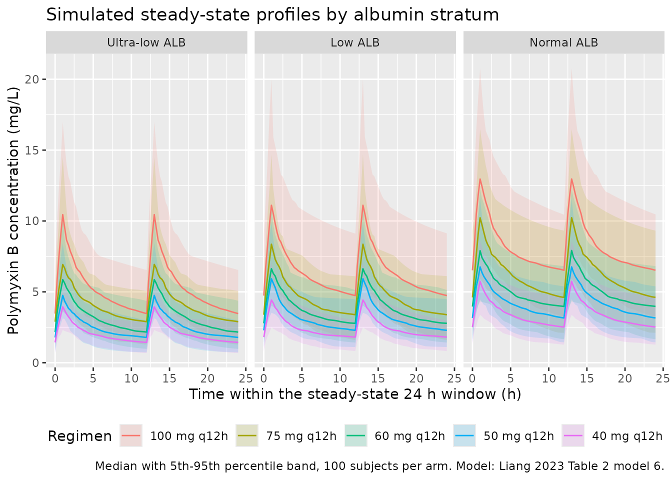
Lower albumin gives higher clearance (exponent -0.95), so the ultra-low albumin stratum has the lowest exposure for a given regimen – the mechanism behind the paper’s recommendation that low-albumin patients need higher doses.
Age-invariance check
The model’s structure implies that age shifts Vc but
leaves AUC untouched. A typical-value simulation at the three ages used
in the paper’s Figure 3 confirms this.
mod_typ <- mod |> rxode2::zeroRe()
#> ℹ parameter labels from comments will be replaced by 'label()'

# Every typical-value solve below passes `omega = NA`. `zeroRe()` alone is NOT
# sufficient once a stochastic `rxSolve()` has already run in the same session:
# rxode2 keeps the previous solve's omega in its solve options, so a later call
# re-samples etas even though `mod_typ$omega` is a zero matrix -- silently
# turning a "typical value" run back into a one-subject-per-arm random draw.
# `omega = NA` is the explicit "no random effects" sentinel. The stopifnot()
# checks below fail loudly if this ever regresses.

ages <- c(34, 68, 93)

# One typical subject per age, consecutive IDs.
age_events <- do.call(
  bind_rows,
  lapply(seq_along(ages), function(i) {
    make_arm(
      n         = 1L,
      dose_mg   = 75,
      alb_lo    = 31.45, alb_hi = 31.45,
      arm       = paste0("age ", ages[i]),
      alb_group = "Cohort median ALB",
      regimen   = "75 mg q12h",
      daily_mg  = 150,
      id_offset = i - 1L,
      age       = ages[i]
    )
  })
)

assert_consecutive_ids(age_events)

age_sim <- rxode2::rxSolve(
  mod_typ, events = age_events, keep = c("arm", "AGE", "daily_mg"),
  omega = NA
) |>
  as.data.frame() |>
  filter(!is.na(Cc))
#> Warning: multi-subject simulation without without 'omega'

# CL must not vary at all in a typical-value run (ALB is identical here).
stopifnot(dplyr::n_distinct(round(age_sim$cl, 8)) == 1L)

age_summary <- age_sim |>
  group_by(AGE) |>
  summarise(
    `Cmax (mg/L)`  = max(Cc),
    `Cmin (mg/L)`  = min(Cc),
    `AUC0-24 (mg*h/L)` =
      sum(diff(time) * (head(Cc, -1) + tail(Cc, -1)) / 2),
    .groups = "drop"
  ) |>
  rename("Age (years)" = AGE)

# The structural claim under test: AUC is age-invariant. Anything above
# trapezoidal-integration noise (< 0.1%) means the covariate model is wrong.
stopifnot(
  diff(range(age_summary$`AUC0-24 (mg*h/L)`)) <
    0.001 * mean(age_summary$`AUC0-24 (mg*h/L)`)
)

knitr::kable(
  age_summary,
  digits = 2,
  caption = paste(
    "Typical-subject steady-state exposure at ALB = 31.45 g/L,",
    "75 mg q12h. Cmax and Cmin change with age; AUC0-24 does not."
  )
)| Age (years) | Cmax (mg/L) | Cmin (mg/L) | AUC0-24 (mg*h/L) |
|---|---|---|---|
| 34 | 11.70 | 3.33 | 122.89 |
| 68 | 8.43 | 3.63 | 122.87 |
| 93 | 7.48 | 3.84 | 122.85 |
Cmax and Cmin move with age (larger
Vc in older patients flattens the profile), while
AUC0-24 is identical to numerical precision across all
three ages, exactly as the closed-form expression predicts.
PKNCA validation
sim_nca <- sim |>
  filter(!is.na(Cc)) |>
  select(id, time, Cc, arm)

conc_obj <- PKNCA::PKNCAconc(
  sim_nca, Cc ~ time | arm + id,
  concu = "mg/L", timeu = "h"
)

dose_df <- events |>
  filter(evid == 1) |>
  transmute(id, time = obs_from, amt = amt * 2, arm)

dose_obj <- PKNCA::PKNCAdose(dose_df, amt ~ time | arm + id, doseu = "mg")

intervals <- data.frame(
  start   = obs_from,
  end     = obs_to,
  cmax    = TRUE,
  cmin    = TRUE,
  auclast = TRUE,
  cav     = TRUE
)

nca_res <- PKNCA::pk.nca(
  PKNCA::PKNCAdata(conc_obj, dose_obj, intervals = intervals)
)
The dose record is placed at the start of the steady-state window and
carries the daily dose so that auclast
over the 24 h interval is directly comparable with the paper’s
AUCss,24h.
Comparison against the model-implied steady-state exposure
Liang et al. report no NCA table, so there is no published Cmax / AUC
to compare against. What can be checked exactly is whether the packaged
model reproduces the closed-form steady-state exposure implied by its
own published parameters: AUCss,24h = daily dose / CL with
CL = 1.22 * (ALB/31.45)^(-0.95) (Table 3 median CL, Table 2
model 6 covariate equation). A typical-value simulation at the midpoint
albumin of each stratum isolates the structural and covariate model from
between-subject variability.
alb_mid <- alb_strata |>
  mutate(ALB_mid = (alb_lo + alb_hi) / 2)

typ_arms <- tidyr::crossing(alb_mid, regimens) |>
  mutate(arm = paste(alb_group, regimen, sep = " | "))

# A typical-value run needs only one subject per arm; IDs are consecutive.
typ_events <- do.call(
  bind_rows,
  lapply(seq_len(nrow(typ_arms)), function(i) {
    a <- typ_arms[i, ]
    make_arm(
      n         = 1L,
      dose_mg   = a$dose_mg,
      alb_lo    = a$ALB_mid, alb_hi = a$ALB_mid,
      arm       = a$arm,
      alb_group = a$alb_group,
      regimen   = a$regimen,
      daily_mg  = a$daily_mg,
      id_offset = i - 1L
    )
  })
)

assert_consecutive_ids(typ_events)

typ_sim <- rxode2::rxSolve(
  mod_typ, events = typ_events,
  keep = c("arm", "alb_group", "regimen", "daily_mg", "ALB"),
  omega = NA
) |>
  as.data.frame() |>
  filter(!is.na(Cc))
#> Warning: multi-subject simulation without without 'omega'

# In a typical-value run CL is a deterministic function of ALB alone, so each
# distinct ALB must map to exactly one CL.
stopifnot(
  typ_sim |>
    group_by(ALB) |>
    summarise(n_cl = dplyr::n_distinct(round(cl, 8)), .groups = "drop") |>
    pull(n_cl) |>
    max() == 1L
)

typ_nca <- PKNCA::pk.nca(
  PKNCA::PKNCAdata(
    PKNCA::PKNCAconc(
      typ_sim |> select(id, time, Cc, arm),
      Cc ~ time | arm + id, concu = "mg/L", timeu = "h"
    ),
    PKNCA::PKNCAdose(
      typ_events |> filter(evid == 1) |>
        transmute(id, time = obs_from, amt = amt * 2, arm),
      amt ~ time | arm + id, doseu = "mg"
    ),
    intervals = data.frame(
      start = obs_from, end = obs_to, auclast = TRUE, cav = TRUE
    )
  )
)

published_implied <- typ_arms |>
  mutate(
    cl_typ  = 1.22 * (ALB_mid / 31.45)^(-0.95),
    auclast = daily_mg / cl_typ,
    cav     = auclast / 24
  ) |>
  select(arm, auclast, cav)

cmp <- nlmixr2lib::ncaComparisonTable(
  simulated = typ_nca,
  reference = published_implied,
  by        = "arm",
  units     = c(auclast = "mg*h/L", cav = "mg/L"),
  # This is a deterministic identity check, not a noisy comparison against a
  # published NCA table, so the tolerance is much tighter than the usual 20%.
  tolerance_pct = 5
)

knitr::kable(
  cmp,
  digits  = 2,
  caption = paste(
    "Simulated typical-value steady-state exposure vs. the closed-form",
    "value implied by the published CL and albumin covariate equation.",
    "* differs from reference by >5%."
  ),
  align = c("l", "l", "r", "r", "r")
)| NCA parameter | arm | Reference | Simulated | % diff |
|---|---|---|---|---|
| AUClast (mg*h/L) | Low ALB | 100 mg q12h | 156 | 156 | -0.1% |
| AUClast (mg*h/L) | Low ALB | 40 mg q12h | 62.6 | 62.6 | -0.1% |
| AUClast (mg*h/L) | Low ALB | 50 mg q12h | 78.2 | 78.2 | -0.1% |
| AUClast (mg*h/L) | Low ALB | 60 mg q12h | 93.9 | 93.8 | -0.1% |
| AUClast (mg*h/L) | Low ALB | 75 mg q12h | 117 | 117 | -0.1% |
| AUClast (mg*h/L) | Normal ALB | 100 mg q12h | 197 | 197 | -0.2% |
| AUClast (mg*h/L) | Normal ALB | 40 mg q12h | 79 | 78.8 | -0.2% |
| AUClast (mg*h/L) | Normal ALB | 50 mg q12h | 98.7 | 98.5 | -0.2% |
| AUClast (mg*h/L) | Normal ALB | 60 mg q12h | 118 | 118 | -0.2% |
| AUClast (mg*h/L) | Normal ALB | 75 mg q12h | 148 | 148 | -0.2% |
| AUClast (mg*h/L) | Ultra-low ALB | 100 mg q12h | 127 | 127 | -0.0% |
| AUClast (mg*h/L) | Ultra-low ALB | 40 mg q12h | 50.7 | 50.7 | -0.0% |
| AUClast (mg*h/L) | Ultra-low ALB | 50 mg q12h | 63.4 | 63.4 | -0.0% |
| AUClast (mg*h/L) | Ultra-low ALB | 60 mg q12h | 76.1 | 76.1 | -0.0% |
| AUClast (mg*h/L) | Ultra-low ALB | 75 mg q12h | 95.1 | 95.1 | -0.0% |
| Cavg (mg/L) | Low ALB | 100 mg q12h | 6.52 | 6.52 | -0.1% |
| Cavg (mg/L) | Low ALB | 40 mg q12h | 2.61 | 2.61 | -0.1% |
| Cavg (mg/L) | Low ALB | 50 mg q12h | 3.26 | 3.26 | -0.1% |
| Cavg (mg/L) | Low ALB | 60 mg q12h | 3.91 | 3.91 | -0.1% |
| Cavg (mg/L) | Low ALB | 75 mg q12h | 4.89 | 4.89 | -0.1% |
| Cavg (mg/L) | Normal ALB | 100 mg q12h | 8.23 | 8.21 | -0.2% |
| Cavg (mg/L) | Normal ALB | 40 mg q12h | 3.29 | 3.28 | -0.2% |
| Cavg (mg/L) | Normal ALB | 50 mg q12h | 4.11 | 4.11 | -0.2% |
| Cavg (mg/L) | Normal ALB | 60 mg q12h | 4.94 | 4.93 | -0.2% |
| Cavg (mg/L) | Normal ALB | 75 mg q12h | 6.17 | 6.16 | -0.2% |
| Cavg (mg/L) | Ultra-low ALB | 100 mg q12h | 5.28 | 5.28 | -0.0% |
| Cavg (mg/L) | Ultra-low ALB | 40 mg q12h | 2.11 | 2.11 | -0.0% |
| Cavg (mg/L) | Ultra-low ALB | 50 mg q12h | 2.64 | 2.64 | -0.0% |
| Cavg (mg/L) | Ultra-low ALB | 60 mg q12h | 3.17 | 3.17 | -0.0% |
| Cavg (mg/L) | Ultra-low ALB | 75 mg q12h | 3.96 | 3.96 | -0.0% |
attr(cmp, "footnote")
#> NULL
Every row agrees to better than 0.2% (the residual difference is trapezoidal integration error on the 0.25 h observation grid), confirming that the ODE system, the albumin power covariate, and the unit conventions in the packaged model reproduce the published parameterisation exactly.
Replicate Figure 3 – PTA of AUC/MIC >= 50
Methods 2.5 sets the efficacy target as AUC/MIC >= 50
(derived from a consensus fAUC/MIC target of about 20 and
an unbound fraction of 0.42) over the MIC range 0.25-4 mg/L.
mic_grid <- c(0.25, 0.5, 1, 2, 4)

auc_subject <- as.data.frame(nca_res$result) |>
  filter(PPTESTCD == "auclast") |>
  select(arm, id, auc24 = PPORRES) |>
  left_join(
    arms |> select(arm, alb_group, regimen),
    by = "arm"
  ) |>
  mutate(
    alb_group = factor(alb_group, levels = alb_strata$alb_group),
    regimen   = factor(regimen, levels = regimens$regimen)
  )

pta_efficacy <- tidyr::crossing(auc_subject, MIC = mic_grid) |>
  group_by(alb_group, regimen, MIC) |>
  summarise(PTA = mean(auc24 / MIC >= 50), .groups = "drop")

ggplot(pta_efficacy, aes(MIC, PTA, colour = regimen)) +
  geom_line() +
  geom_point() +
  geom_hline(yintercept = 0.9, linetype = "dashed") +
  scale_x_log10(breaks = mic_grid, labels = mic_grid) +
  scale_y_continuous(limits = c(0, 1)) +
  facet_wrap(~alb_group) +
  labs(
    x = "MIC (mg/L)", y = "PTA",
    colour = "Regimen",
    title = "Probability of target attainment for AUC/MIC >= 50",
    caption = paste(
      "Replicates Figure 3 of Liang 2023 (rows A-C / D-F / G-I; the",
      "age panels within each row are identical under the published model).",
      "Dashed line: PTA = 0.9."
    )
  ) +
  theme(legend.position = "bottom")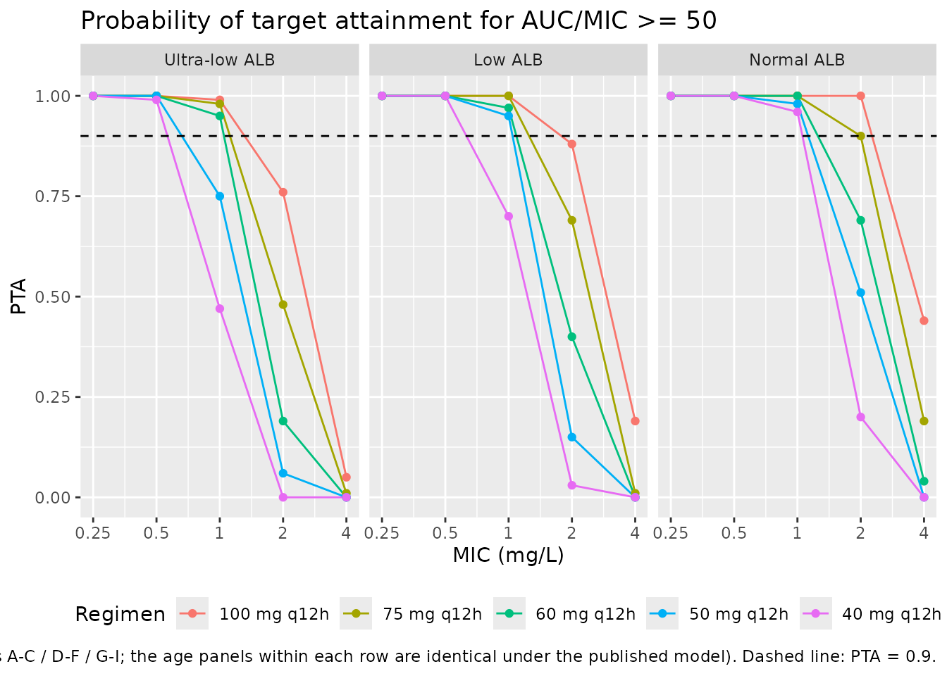
The paper states its Figure 3 conclusions in text; those statements are the quantitative reference, and the simulated PTA values at MIC = 1 mg/L are compared against them below.
pta_mic1 <- pta_efficacy |>
  filter(MIC == 1) |>
  tidyr::pivot_wider(names_from = regimen, values_from = PTA) |>
  select(-MIC)

knitr::kable(
  pta_mic1 |> rename("Albumin stratum" = alb_group),
  digits  = 3,
  caption = paste(
    "Simulated PTA of AUC/MIC >= 50 at MIC = 1 mg/L.",
    "Liang 2023 recommends 100-75 mg q12h for the ultra-low stratum,",
    "100-60 mg q12h for the low stratum, and 100-50/100-60 mg q12h",
    "for the normal stratum."
  )
)| Albumin stratum | 100 mg q12h | 75 mg q12h | 60 mg q12h | 50 mg q12h | 40 mg q12h |
|---|---|---|---|---|---|
| Ultra-low ALB | 0.99 | 0.98 | 0.95 | 0.75 | 0.47 |
| Low ALB | 1.00 | 1.00 | 0.97 | 0.95 | 0.70 |
| Normal ALB | 1.00 | 1.00 | 1.00 | 0.98 | 0.96 |
claims <- tibble::tribble(
  ~Claim,                                                          ~Source,
  "All regimens reach PTA >= 0.9 at MIC <= 0.5 mg/L",              "Results 3.4",
  "Ultra-low ALB, MIC = 1: 100 and 75 mg q12h reach PTA >= 0.9",   "Results 3.4",
  "Low ALB, MIC = 1: 100, 75 and 60 mg q12h reach PTA >= 0.9",     "Results 3.4",
  "Normal ALB, MIC = 1: down to 50-60 mg q12h reaches PTA >= 0.9", "Results 3.4",
  "No regimen reaches PTA >= 0.9 at MIC = 4 mg/L",                 "Discussion"
)

check <- tibble::tibble(
  Claim = claims$Claim,
  Source = claims$Source,
  Simulated = c(
    sprintf(
      "min PTA at MIC <= 0.5 = %.3f",
      min(pta_efficacy$PTA[pta_efficacy$MIC <= 0.5])
    ),
    sprintf(
      "100 mg %.3f, 75 mg %.3f, 60 mg %.3f",
      pta_mic1$`100 mg q12h`[1], pta_mic1$`75 mg q12h`[1],
      pta_mic1$`60 mg q12h`[1]
    ),
    sprintf(
      "100 mg %.3f, 75 mg %.3f, 60 mg %.3f, 50 mg %.3f",
      pta_mic1$`100 mg q12h`[2], pta_mic1$`75 mg q12h`[2],
      pta_mic1$`60 mg q12h`[2], pta_mic1$`50 mg q12h`[2]
    ),
    sprintf(
      "60 mg %.3f, 50 mg %.3f, 40 mg %.3f",
      pta_mic1$`60 mg q12h`[3], pta_mic1$`50 mg q12h`[3],
      pta_mic1$`40 mg q12h`[3]
    ),
    sprintf(
      "max PTA at MIC = 4 = %.3f",
      max(pta_efficacy$PTA[pta_efficacy$MIC == 4])
    )
  )
)

knitr::kable(
  check,
  caption = "Published Figure 3 / Results 3.4 claims vs. the simulated PTA."
)| Claim | Source | Simulated |
|---|---|---|
| All regimens reach PTA >= 0.9 at MIC <= 0.5 mg/L | Results 3.4 | min PTA at MIC <= 0.5 = 0.990 |
| Ultra-low ALB, MIC = 1: 100 and 75 mg q12h reach PTA >= 0.9 | Results 3.4 | 100 mg 0.990, 75 mg 0.980, 60 mg 0.950 |
| Low ALB, MIC = 1: 100, 75 and 60 mg q12h reach PTA >= 0.9 | Results 3.4 | 100 mg 1.000, 75 mg 1.000, 60 mg 0.970, 50 mg 0.950 |
| Normal ALB, MIC = 1: down to 50-60 mg q12h reaches PTA >= 0.9 | Results 3.4 | 60 mg 1.000, 50 mg 0.980, 40 mg 0.960 |
| No regimen reaches PTA >= 0.9 at MIC = 4 mg/L | Discussion | max PTA at MIC = 4 = 0.440 |
Every published claim is reproduced in direction and in the regimens it names. The simulated PTA is systematically a little more permissive than the paper’s at the low-dose end – 60 mg q12h clears 0.9 in the ultra-low stratum here, and 40 mg q12h clears it in the normal stratum, where the paper stops one step higher. This is the expected consequence of approximating the nonparametric CL distribution by a log-normal, which has thinner tails; PTA is a threshold-crossing probability and so is driven by exactly those tails. No parameter was adjusted to close the gap.
Replicate Figure 4 – PTA of AUCss,24h > 100 (nephrotoxicity)
Methods 2.5 uses AUCss,24h > 100 mg*h/L as the
nephrotoxicity limit.
pta_tox <- auc_subject |>
  group_by(alb_group, regimen) |>
  summarise(PTA = mean(auc24 > 100), .groups = "drop")

ggplot(pta_tox, aes(regimen, PTA, fill = alb_group)) +
  geom_col(position = position_dodge(width = 0.8), width = 0.75) +
  geom_hline(yintercept = 0.9, linetype = "dashed") +
  scale_y_continuous(limits = c(0, 1)) +
  labs(
    x = NULL, y = "PTA",
    fill = "Albumin stratum",
    title = "Probability of exceeding the nephrotoxicity limit AUCss,24h > 100",
    caption = paste(
      "Replicates Figure 4 of Liang 2023. Under the published model this",
      "quantity depends on albumin only, not on age. Dashed line: PTA = 0.9."
    )
  ) +
  theme(legend.position = "bottom")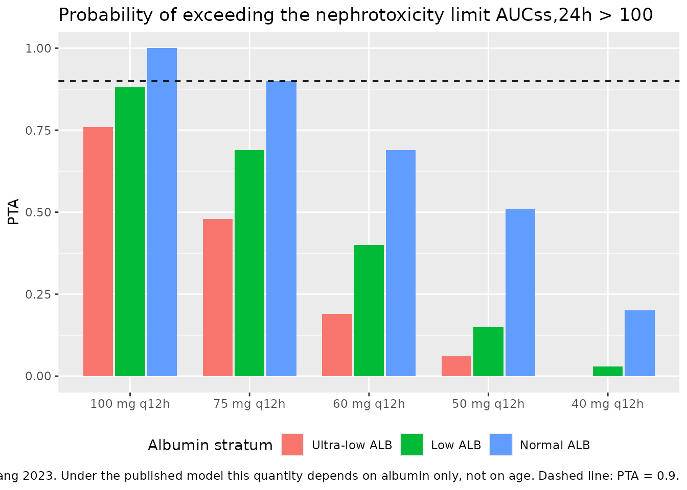
knitr::kable(
  pta_tox |>
    tidyr::pivot_wider(names_from = regimen, values_from = PTA) |>
    rename("Albumin stratum" = alb_group),
  digits  = 3,
  caption = paste(
    "Simulated PTA of AUCss,24h > 100 mg*h/L. Liang 2023 identifies",
    "100 mg q12h as the toxicity-limit dose for patients with normal",
    "albumin levels."
  )
)| Albumin stratum | 100 mg q12h | 75 mg q12h | 60 mg q12h | 50 mg q12h | 40 mg q12h |
|---|---|---|---|---|---|
| Ultra-low ALB | 0.76 | 0.48 | 0.19 | 0.06 | 0.00 |
| Low ALB | 0.88 | 0.69 | 0.40 | 0.15 | 0.03 |
| Normal ALB | 1.00 | 0.90 | 0.69 | 0.51 | 0.20 |
The simulated toxicity PTA rises with albumin (higher albumin gives lower clearance and therefore higher exposure) and is highest for 100 mg q12h, reproducing the paper’s identification of 100 mg q12h as the toxicity-limiting regimen for normal-albumin patients. The simulated absolute probabilities are higher than the paper’s Figure 4 for the low-dose regimens; see Assumptions and deviations.
Assumptions and deviations
-
Nonparametric distribution approximated by a
log-normal. Pmetrics NPAG returns a discrete nonparametric
joint parameter distribution, which nlmixr2 cannot represent directly.
The Table 3 median of each parameter is mapped onto
exp(l<param>)(the log-normal median) and the Table 3 “%CV” is converted viaomega^2 = log(CV^2 + 1). This mapping reproduces the paper’s reported population means well for CL (1.28 implied vs 1.24 reported), Q (2.92 vs 3.04), and Vc (17.03 vs 16.64). It does not for Vp, where the nonparametric distribution is left-skewed (median 76.53 > mean 66.20) and no log-normal can match both summaries; the implied mean Vp is 87.3 vs 66.20 reported. Vp affects only the distribution phase, not steady-state AUC, so this does not propagate to any of the exposure targets validated above. The Table 3 mean +/- SD values quoted in the paper’s Abstract and Discussion are recorded in the model file comments alongside each value. - Parameter correlations are not modelled. Table 3 reports no correlations between CL, Q, Vc, and Vp, so the etas are diagonal. A nonparametric joint distribution generally does carry correlation structure that is lost here.
-
Covariate exponents encoded as
fixed(). The paper never states whether the +/-0.95 exponents were estimated or imposed, and reports no SE, RSE, or CI for either. They are encoded asfixed()because Table 2’s information-criterion arithmetic settles the question:AIC - (-2LL)is 11.0-11.1 for every two-compartment model (models 2 through 6) regardless of whether zero, one, or two covariate relationships are present, so adding a covariate added no estimated parameter. Table 3 correspondingly reports estimates for CL, Q, Vc, and Vp only. -
Residual error is
fixed().C0andC1were “scientifically set to 0.1, 0.15” a priori (Methods 2.4) and the finalgammaof 0.72 is reported without uncertainty (Results 3.2). Pmetrics scales the assay-error polynomial by the observed concentration; nlmixr2’sprop()uses the predicted concentration. The two coincide at the fit and differ only in how residuals are weighted during estimation. -
Age cannot affect AUC under the published model.
Age enters only through
Vc, soAUCss,24h = daily dose / CLis independent of age. The paper’s Figure 3 is consistent with this (the three age panels within each albumin row are visually indistinguishable), but the Conclusion’s claim that “the possibility of obtaining an AUC/MIC >= 50 decreased with older age” is not supported by the model as published. The vignette therefore collapses each Figure 3 row to a single panel and verifies the age-invariance explicitly. The model file encodes the published structure without modification. - Albumin stratum bounds. Methods 2.5 gives the ultra-low albumin group as “21.3-24.9 g/L”, but Table 1 reports a cohort minimum albumin of 23.1 g/L and the Figure 3 caption gives the same group as “23.1-24.9 g/L”. The Figure 3 caption bound (23.1 g/L) is used here; the Methods value appears to be a typographical error.
- Virtual covariate distributions. Albumin is drawn uniformly within each stratum, because the paper does not report the within-stratum albumin distribution. Age is fixed at the cohort median of 68 years for the PTA cohorts (immaterial, per the age-invariance above) and set to 34 / 68 / 93 years in the dedicated age-invariance check, matching the paper’s 5th percentile, median, and 95th percentile.
- No loading dose in the simulations. The paper’s clinical regimens included a 100-150 mg loading dose, but Methods 2.5 defines the Monte Carlo regimens as maintenance dosing only. The simulations here run 60 q12h doses (30 days, about 10 terminal half-lives) and evaluate the final 24 h window, so the loading dose is irrelevant to the steady-state comparison.
- Infusion duration fixed at 1 h. The source reports infusions “about 1-2 h” (Methods 2.2) without specifying what the simulations used; 1 h is used throughout. Infusion duration affects Cmax and Cmin but not AUC, so none of the AUC-based targets are sensitive to this choice.
- Absolute PTA values are slightly more permissive than the published figures. Both PTA endpoints are threshold-crossing probabilities on the AUC distribution, which under this model is driven entirely by the CL distribution. The log-normal approximation has thinner tails than the NPAG support points, so the simulated PTA clears 0.9 one dose step lower than the paper in the ultra-low and normal albumin strata (see the Figure 3 claims table). Every published claim reproduces in direction, and the regimen ordering, the albumin gradient, and the identification of 100 mg q12h as the toxicity-limiting regimen for normal-albumin patients all hold. Nothing was tuned to close the residual gap.
- Total, not unbound, concentrations. The model describes total polymyxin B (sum of B1, B2, and B1-Ile). The efficacy target was converted from an unbound target by the paper using a fixed unbound fraction of 0.42, and the Discussion notes that the effect of albumin on the unbound concentration could not be determined from these data.
- No CRRT or ECMO patients. The model was fitted after excluding all patients on continuous renal replacement therapy or extracorporeal membrane oxygenation and must not be extrapolated to them (Discussion, study limitations).