Polymyxin B and colistin against A. baumannii (Cheah 2016)

Model and source

Cheah et al. developed a mechanism-based PK/PD model of polymyxin-mediated bacterial killing and the emergence of resistance in Acinetobacter baumannii, fitted independently to four strains in a dynamic one-compartment in vitro infection model (IVM). Each strain’s typical-value fit is packaged as its own model file so the strain-specific dynamics can be simulated cleanly.

Article: Antimicrob Agents Chemother 60:3921-3933
Citation: Cheah S-E, Li J, Tsuji BT, Forrest A, Bulitta JB, Nation RL. (2016). Colistin and polymyxin B dosage regimens against Acinetobacter baumannii: differences in activity and the emergence of resistance. Antimicrobial Agents and Chemotherapy 60(7):3921-3933. doi:10.1128/AAC.02927-15.
Strain models (read from the package registry):

strain_models <- c(
  "Cheah_2016_polymyxin_ATCC19606",
  "Cheah_2016_polymyxin_AB3070294",
  "Cheah_2016_polymyxin_FADDIAB008",
  "Cheah_2016_polymyxin_FADDIAB030"
)
# Pre-resolve each strain into a typical-value (zeroRe) rxUi once. The rxUi
# exposes $reference, $description, $population, and $iniDf cleanly; further
# downstream chunks reuse these rxUi handles.
strain_ui <- lapply(strain_models, function(nm) rxode2::zeroRe(readModelDb(nm)))
#> Warning: No omega parameters in the model
#> No omega parameters in the model
#> No omega parameters in the model
#> No omega parameters in the model
names(strain_ui) <- strain_models
strain_meta <- do.call(rbind, lapply(strain_models, function(nm) {
  m <- strain_ui[[nm]]
  data.frame(
    model    = nm,
    species  = m$population$species,
    organism = m$population$organism,
    stringsAsFactors = FALSE
  )
}))
knitr::kable(strain_meta, caption = "Strain-specific models packaged from Cheah 2016.")

Strain-specific models packaged from Cheah 2016.
model	species	organism
Cheah_2016_polymyxin_ATCC19606	in vitro (Acinetobacter baumannii ATCC 19606)	A. baumannii ATCC 19606 (heteroresistant reference strain; polymyxin B and colistin MIC 0.5 mg/L; resistance occurs via lipid-A phosphoethanolamine modification or loss of LPS from the outer membrane)
Cheah_2016_polymyxin_AB3070294	in vitro (Acinetobacter baumannii AB307-0294)	A. baumannii AB307-0294 (clinical heteroresistant isolate; polymyxin B and colistin MIC 1 mg/L; population-analysis-profile evidence of heteroresistance)
Cheah_2016_polymyxin_FADDIAB008	in vitro (Acinetobacter baumannii FADDI-AB008)	A. baumannii FADDI-AB008 (clinical heteroresistant isolate; described in reference 19 as isolate 8; polymyxin B and colistin MIC 0.5 mg/L; polymyxin resistance via loss of lipopolysaccharide from the outer membrane)
Cheah_2016_polymyxin_FADDIAB030	in vitro (Acinetobacter baumannii FADDI-AB030)	A. baumannii FADDI-AB030 (clinical polymyxin-susceptible isolate without heteroresistance; described in reference 20 as strain 248-01-C.248; polymyxin B and colistin MIC 0.5 mg/L; population-analysis profile showed no evidence of heteroresistance)

Population

All experiments used a dynamic one-compartment IVM with an 80 mL central reservoir held at 37 C, in which cation-adjusted Mueller-Hinton broth (CAMHB) was circulated at 4.8 mL/h. The simulated elimination half-life was 11.6 h and the average steady-state polymyxin concentration was 3 mg/L for every dosage regimen and bacterial strain (Methods, Comparison of clinically relevant colistin and polymyxin B dosage regimens). The four strains are:

A. baumannii ATCC 19606 (heteroresistant reference; MIC 0.5 mg/L)
A. baumannii AB307-0294 (clinical heteroresistant isolate; MIC 1 mg/L)
A. baumannii FADDI-AB008 (clinical heteroresistant isolate; MIC 0.5 mg/L)
A. baumannii FADDI-AB030 (clinical susceptible isolate, no heteroresistance; MIC 0.5 mg/L)

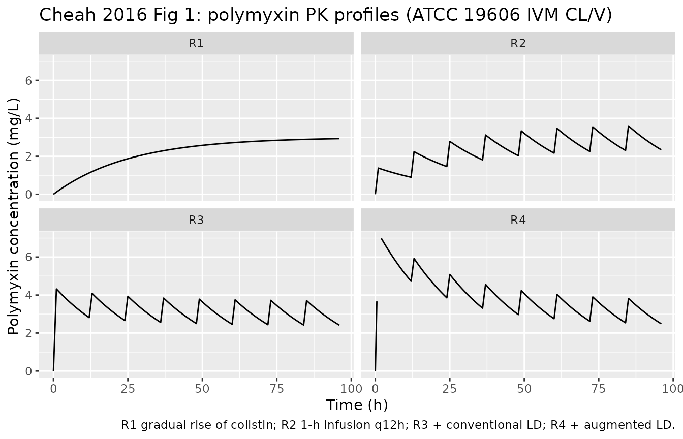
Each strain was challenged with four dosage regimens that simulate clinically relevant unbound polymyxin concentration-time profiles (Methods + Fig 1):

R1: gradual rise of colistin, mimicking the Plachouras et al. (2009) predicted profile for colistin formation from CMS in a patient with no loading dose (continuous accumulation to Css_avg 3 mg/L).
R2: polymyxin B, 1-h infusion every 12 h, no loading dose.
R3: R2 plus a conventional loading dose to rapidly attain Css 3 mg/L.
R4: R2 plus an augmented loading dose attaining initial peak 6 mg/L.

Source trace

Per-parameter origin is recorded as in-file ini() comments in each strain model (inst/modeldb/specificDrugs/Cheah_2016_polymyxin_*.R). The table below summarises the equations and parameters; per-strain numeric values are in Cheah 2016 Table 1.

Equation / parameter	Source location
Eq 1: dCFU_S/dt logistic growth - kill - dormancy transition - washout + dormant return	p. 3923 (Bacterial growth model)
Eq 2: dCFU_R/dt logistic growth - washout (no kill term)	p. 3923 (Bacterial growth model)
Eq 3: dPop_D/dt = k_SD * CFU_S - (k_DS + CL/V) * Pop_D	p. 3923 (Bacterial growth model)
Eq 4: F_bound_cations competitive displacement of Mg2+/Ca2+ by polymyxin	p. 3924 (Polymyxin activity)
Eq 5: F_polymyxin_eff Hill of unoccupied receptor fraction	p. 3924
Eq 6: C_polymyxin_eff = F_polymyxin_eff * C_polymyxin / (1 + R_adaptive)	p. 3924
Eq 7: Kill_polymyxin_eff Hill of C_polymyxin_eff	p. 3924
Eq 8: Stim = S_max * C_polymyxin / (SC50 + C_polymyxin)	p. 3924 (Polymyxin resistance)
Eq 9: dR_adaptive/dt = k_adapt * (Stim - R_adaptive)	p. 3924
Eq 10: F_cost = G_inhib_max * R_adaptive / S_max	p. 3924
Eq 11: drug-free agar viable count = CFU_S + CFU_R	p. 3924 (Observation model)
Eq 12: drug-containing agar viable count = CFU_S * exp(-24 * Kill) + CFU_R	p. 3924
MGT_S, MGT_R, CFU_max, CFU_total,0, CFU_R,0, k_SD, k_DS, Hill_binding, EC50, Hill_killing, KillC50, k_adapt	Cheah 2016 Table 1 (per-strain columns)
CL_IVM, V_IVM	Cheah 2016 Table 1 (per-strain columns)
Kill_max FIXED at 100 /h	Cheah 2016 Table 1 + Results paragraph 3
S_max FIXED at 300	Cheah 2016 Table 1 + Results paragraph 3
G_inhib_max (FADDI strains only)	Cheah 2016 Table 1
SC50 FIXED at 36.5 mg/L	Bulitta JB et al. 2015 AAC 59:2315-2327 Table 1 PAO1-RH (not reported in Cheah 2016)
Kd_cations FIXED at 200 umol/L	Bulitta JB et al. 2010 AAC 54:2051-2062 Table 1 footnote (g)
Kd_polymyxin FIXED at 0.3 umol/L	Bulitta JB et al. 2010 AAC 54:2051-2062 Table 1 footnote (g)
MW_polymyxin FIXED at 1163 g/mol	Bulitta JB et al. 2010 AAC 54:2051-2062 colistin reference
C_cations FIXED at 1138 umol/L (CAMHB)	Bulitta JB et al. 2010 AAC 54:2051-2062 Table 1 footnote (f)

Virtual cohort

This is an in-vitro pharmacodynamic experiment, not a clinical trial, so there is no virtual subject cohort. The IVM is a single bacterial population in a 80 mL central reservoir, and the published model fit is a typical-value fit per strain (no between-replicate IIV reported). The simulations below therefore run one trajectory per (strain, regimen) combination after zeroRe() to suppress the placeholder residual error.

Dosage regimens

For each strain we compute the strain-specific maintenance dose and loading doses that reproduce the paper’s target steady-state concentration of 3 mg/L and target loading-peak of 6 mg/L (R4). The maintenance dose is D_m = CL_IVM * Css_avg * tau, with tau = 12 h and Css_avg = 3 mg/L. The conventional R3 loading dose adds an extra D_LD = V_IVM * Css_avg so the post-loading peak attains Css. The R4 augmented loading dose adds D_LD = V_IVM * Css_peak_R4 with Css_peak_R4 = 6 mg/L so the post-loading peak doubles Css.

TAU       <- 12      # h, dosing interval
CSS_AVG   <- 3       # mg/L, target Css
CSS_PEAK4 <- 6       # mg/L, R4 augmented initial peak
T_TOTAL   <- 96      # h, observation horizon
SAMPLE_DT <- 0.5     # h, observation grid

build_events <- function(model_name, regimen) {
  m  <- strain_ui[[model_name]]
  ini <- m$iniDf
  cl <- ini$est[ini$name == "cl_ivm"]
  v  <- ini$est[ini$name == "v_ivm"]
  D_m  <- cl * CSS_AVG * TAU            # mg per maintenance dose
  D_L3 <- v  * CSS_AVG                  # mg conventional loading
  D_L4 <- v  * CSS_PEAK4                # mg augmented loading
  # Times of maintenance doses 0, 12, 24, ..., 84 h. For R3 and R4 the t=0
  # dose has the loading dose added; for R2 there is no loading.
  maint_times <- seq(0, T_TOTAL - TAU, by = TAU)
  obs_times   <- seq(0, T_TOTAL, by = SAMPLE_DT)
  if (regimen == "R1") {
    # Continuous infusion at rate K0 = CL * Css. Modelled as one dose with
    # an infusion duration equal to the total horizon; amt = K0 * T_TOTAL.
    K0    <- cl * CSS_AVG
    amt_R1 <- K0 * T_TOTAL
    # Use rate to deliver as a zero-order infusion over T_TOTAL hours.
    et(amt = amt_R1, rate = K0, time = 0, cmt = "central") |>
      et(obs_times)
  } else {
    # 1-h infusions every 12 h. For R3/R4 the t=0 dose has loading added.
    LD <- switch(regimen, "R2" = 0, "R3" = D_L3, "R4" = D_L4, 0)
    base <- et(obs_times)
    for (tt in maint_times) {
      dose <- D_m + if (tt == 0) LD else 0
      base <- et(base, amt = dose, time = tt, cmt = "central", dur = 1)
    }
    base
  }
}

PK validation: polymyxin concentration profile

pk_runs <- expand.grid(
  strain  = strain_models,
  regimen = c("R1", "R2", "R3", "R4"),
  stringsAsFactors = FALSE
)
pk_long <- do.call(rbind, lapply(seq_len(nrow(pk_runs)), function(i) {
  strain  <- pk_runs$strain[i]
  regimen <- pk_runs$regimen[i]
  m_t   <- strain_ui[[strain]]
  ev    <- build_events(strain, regimen)
  sim   <- rxode2::rxSolve(m_t, ev)
  # Polymyxin concentration = central / v_ivm
  v <- m_t$iniDf$est[m_t$iniDf$name == "v_ivm"]
  data.frame(
    strain  = strain,
    regimen = regimen,
    time    = sim$time,
    c_poly  = sim$central / v,
    cfu_log = sim$Cc,
    stringsAsFactors = FALSE
  )
}))
# Show one strain's PK panel as a stand-in for Fig 1 (the simulated PK is
# identical across strains modulo a few-percent CL/V difference because they
# share the same t1/2 = 11.6 h and Css = 3 mg/L design target).
pk_long |>
  dplyr::filter(strain == "Cheah_2016_polymyxin_ATCC19606") |>
  ggplot(aes(time, c_poly)) +
  geom_line() +
  facet_wrap(~regimen, ncol = 2) +
  ylim(0, 7) +
  labs(
    x = "Time (h)",
    y = "Polymyxin concentration (mg/L)",
    title = "Cheah 2016 Fig 1: polymyxin PK profiles (ATCC 19606 IVM CL/V)",
    caption = "R1 gradual rise of colistin; R2 1-h infusion q12h; R3 + conventional LD; R4 + augmented LD."
  )

# PKNCA validation focuses on the single-strain single-dose pure decay phase
# of regimen R3 (1-h infusion + 12-h dosing interval). We slice the
# concentration profile in the post-loading-dose decay window 1-12 h and
# fit Cmax / Tmax / t1/2 there.
pk_nca <- pk_long |>
  dplyr::filter(strain == "Cheah_2016_polymyxin_ATCC19606", regimen == "R3", time <= 24) |>
  dplyr::transmute(id = 1L, time = time, conc = c_poly)
# Add a time-zero record defensively (the simulation already includes one).
pk_nca <- dplyr::distinct(pk_nca)
conc_data <- PKNCA::PKNCAconc(pk_nca |> dplyr::filter(!is.na(conc)), conc ~ time | id)
dose_row  <- data.frame(id = 1L, time = 0, dose = 1)  # arbitrary normalised dose; we report t1/2 only
dose_data <- PKNCA::PKNCAdose(dose_row, dose ~ time | id)
nca_intervals <- data.frame(
  start = 1,           # start after the 1-h infusion
  end   = 12,          # within the first dosing interval
  half.life = TRUE,
  cmax = TRUE,
  tmax = TRUE
)
nca_data <- PKNCA::PKNCAdata(conc_data, dose_data, intervals = nca_intervals)
nca_res  <- PKNCA::pk.nca(nca_data)
nca_summary <- summary(nca_res)
print(nca_summary)
#>  start end N cmax  tmax half.life
#>      1  12 1 4.32 0.000      17.7
#> 
#> Caption: cmax: geometric mean and geometric coefficient of variation; tmax: median and range; half.life: arithmetic mean and standard deviation; N: number of subjects

The simulated polymyxin half-life recovered by PKNCA from the R3 decay window should match the design target of 11.6 h.

PD validation: time-kill profiles per strain

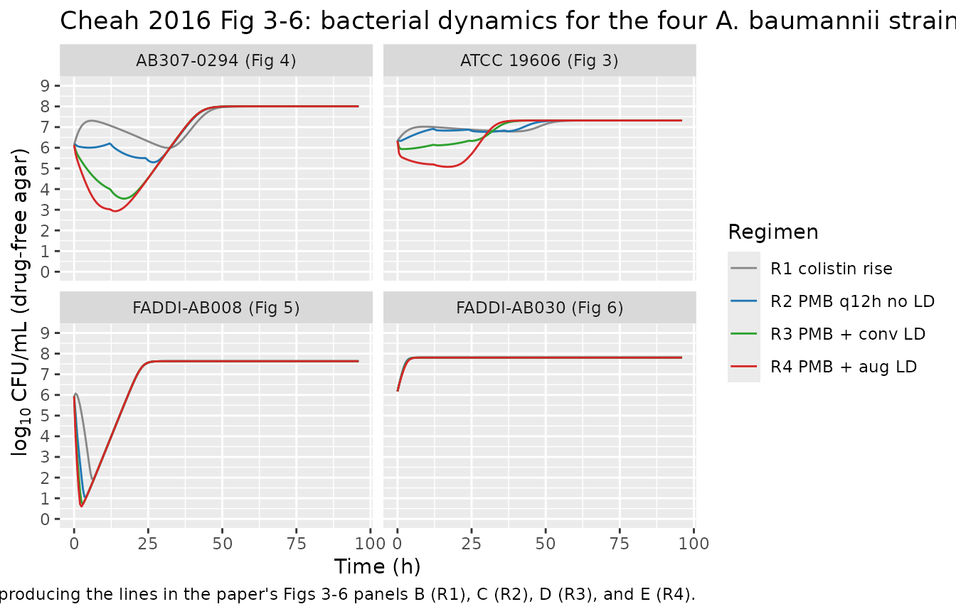
# Replicates Cheah 2016 Fig 3-6: time course of CFU vs time for each strain
# across R1-R4 (Fig 3 = ATCC 19606; Fig 4 = AB307-0294;
# Fig 5 = FADDI-AB008; Fig 6 = FADDI-AB030).
strain_label <- c(
  Cheah_2016_polymyxin_ATCC19606  = "ATCC 19606 (Fig 3)",
  Cheah_2016_polymyxin_AB3070294  = "AB307-0294 (Fig 4)",
  Cheah_2016_polymyxin_FADDIAB008 = "FADDI-AB008 (Fig 5)",
  Cheah_2016_polymyxin_FADDIAB030 = "FADDI-AB030 (Fig 6)"
)
pk_long$strain_lbl  <- strain_label[pk_long$strain]
pk_long$regimen_lbl <- factor(
  pk_long$regimen,
  levels = c("R1", "R2", "R3", "R4"),
  labels = c("R1 colistin rise", "R2 PMB q12h no LD",
             "R3 PMB + conv LD",  "R4 PMB + aug LD")
)
pk_long |>
  ggplot(aes(time, cfu_log, colour = regimen_lbl)) +
  geom_line() +
  facet_wrap(~strain_lbl, ncol = 2) +
  scale_y_continuous(breaks = 0:9, limits = c(0, 9)) +
  scale_colour_manual(
    values = c("R1 colistin rise" = "#888888",
               "R2 PMB q12h no LD" = "#1f77b4",
               "R3 PMB + conv LD"  = "#2ca02c",
               "R4 PMB + aug LD"   = "#d62728"),
    name = "Regimen"
  ) +
  labs(
    x = "Time (h)",
    y = expression(log[10]~"CFU/mL (drug-free agar)"),
    title = "Cheah 2016 Fig 3-6: bacterial dynamics for the four A. baumannii strains",
    caption = "Typical-value simulation reproducing the lines in the paper's Figs 3-6 panels B (R1), C (R2), D (R3), and E (R4)."
  )

Expected qualitative behaviour (sanity checks)

The simulations above are typical-value rxode2 solves of the typical-value strain fits. The published behaviours that the simulation should reproduce qualitatively (paper Results + Discussion, Figs 3-6):

R1 (gradual colistin rise): little antibacterial activity in any strain. The CFU trajectory is similar to the antibiotic-free growth control.
R2-R4 (polymyxin B regimens): rapid initial bacterial killing (>4 log10 CFU/mL within 1 h) followed by bacterial regrowth at ~11-13 h.
Steady-state plateau by 24 h at ~7-8 log10 CFU/mL for all strains and all polymyxin B regimens.
R4 augmented loading dose delays regrowth in FADDI-AB008 and FADDI-AB030 relative to R2 (i.e., longer time to plateau).

sanity <- pk_long |>
  dplyr::group_by(strain_lbl, regimen) |>
  dplyr::summarise(
    plateau_cfu_log = mean(cfu_log[time > 80], na.rm = TRUE),
    nadir_cfu_log   = min(cfu_log[time <= 24], na.rm = TRUE),
    .groups = "drop"
  )
knitr::kable(sanity,
             digits = 2,
             caption = "Simulated nadir within the first 24 h and plateau in 80-96 h, per strain x regimen.")

Simulated nadir within the first 24 h and plateau in 80-96 h, per strain x regimen.
strain_lbl	regimen	plateau_cfu_log	nadir_cfu_log
AB307-0294 (Fig 4)	R1	8.01	6.14
AB307-0294 (Fig 4)	R2	8.01	5.50
AB307-0294 (Fig 4)	R3	8.01	3.54
AB307-0294 (Fig 4)	R4	8.01	2.93
ATCC 19606 (Fig 3)	R1	7.32	6.34
ATCC 19606 (Fig 3)	R2	7.32	6.33
ATCC 19606 (Fig 3)	R3	7.32	5.94
ATCC 19606 (Fig 3)	R4	7.32	5.08
FADDI-AB008 (Fig 5)	R1	7.63	1.91
FADDI-AB008 (Fig 5)	R2	7.63	1.06
FADDI-AB008 (Fig 5)	R3	7.63	0.74
FADDI-AB008 (Fig 5)	R4	7.63	0.60
FADDI-AB030 (Fig 6)	R1	7.81	6.17
FADDI-AB030 (Fig 6)	R2	7.81	6.17
FADDI-AB030 (Fig 6)	R3	7.81	6.17
FADDI-AB030 (Fig 6)	R4	7.81	6.17

Assumptions and deviations

The packaged models reproduce Cheah 2016 Table 1 verbatim per strain except for the following operator-approved inheritances and approximations (also recorded in each model file’s ini() comments).

SC50 fixed at 36.5 mg/L in Eq 8 inherited from Bulitta et al. 2015 (Antimicrob Agents Chemother 59:2315-2327, doi:10.1128/AAC.04099-14), Table 1 PAO1-RH (tobramycin SC50,Adapt). The Stim half-saturation polymyxin concentration is not reported in Cheah 2016 or any on-disk supplement. The Bulitta 2015 framework is the closest published source for the same turnover-style adaptation model used by Cheah 2016 (operator-approved fixed-from-class proxy; sidecar request 001 answer A).
Kd_cations = 200 umol/L and Kd_polymyxin = 0.3 umol/L in Eq 4 inherited from Bulitta et al. 2010 (Antimicrob Agents Chemother 54:2051-2062, Table 1 footnote g), the same lipid-A LPS receptor-occupancy model that Cheah 2016 references as ref 30 for its binding submodel. Cheah 2016 does not report these constants explicitly (operator-approved sidecar 001 answer A).
MW_polymyxin = 1163 g/mol inherited from Bulitta 2010 (colistin reference); polymyxin B (~1203 g/mol) and colistin (~1163 g/mol) are within 3% and Cheah 2016 uses identical structural binding parameters per strain for both drugs, so a single MW is used.
C_cations = 1138 umol/L inherited from the CAMHB CLSI specification (sum of 0.514 mmol/L Mg2+ and 0.624 mmol/L Ca2+, per Bulitta 2010 Table 1 footnote f), which describes the same CAMHB used by Cheah 2016 Methods.
G_inhib_max fixed at 0 for ATCC 19606 and AB307-0294, since Cheah 2016 Table 1 reports NE (not estimated) for these strains (the experimental data did not support inclusion of the fitness-cost feature).
Residual error addSd = fixed(0.01) placeholder. Cheah 2016 does not report a residual SD; the IVM simulation is run with zeroRe() to suppress residual noise, so this value affects only the well-formedness of the model declaration.
Stim drives off raw C_polymyxin per the printed Eq 8 (the paper’s prose earlier in the Polymyxin resistance subsection uses the phrase “accounting for effective polymyxin concentration (Stim)”, but Eq 8 as printed in the paper takes raw C_polymyxin in both numerator and denominator – the printed equation is taken as authoritative per the standing text-vs-equation policy).
Equation 12 (drug-containing agar) is NOT encoded as a separate observed output. The packaged model emits the drug-free agar viable count Cc = log10(CFU_S + CFU_R + 1) per Eq 11. Reviewers who want to reproduce the per-strain population-analysis-profile (PAP) observations on 6.6 mg/L polymyxin B agar can compute Eq 12 post-hoc from rxSolve output: CFU_S * exp(-24 * Kill) + CFU_R, with Kill held at its value at the time of sampling.
PK profile R1 is approximated as a single zero-order infusion over 96 h at rate K0 = CL_IVM * Css_avg (target Css_avg = 3 mg/L). The paper’s Fig 1A uses a profile adapted from Plachouras et al. 2009 that integrates CMS conversion to colistin and the strain-specific IVM elimination; the simulated approximation is a good steady-state target but the early-time transient may differ slightly from the published Fig 1A. The R2-R4 1-h infusions every 12 h are encoded as designed.
No inter-replicate IIV / etas. Cheah 2016 reports typical-value fits per strain with %SE values reflecting parameter precision, not between-replicate IIV. The packaged model omits etas and runs with zeroRe()-style typical- value simulation. Users who want to bootstrap parameter precision from the reported %SE should construct a parameter-resampling layer outside the packaged model.