Empagliflozin (Fayette 2023)
Source:vignettes/articles/Fayette_2023_empagliflozin.Rmd
Fayette_2023_empagliflozin.RmdModel and source
- Citation: Fayette L, Sailer MO, Perez-Pitarch A. Pharmacometrics enhanced Bayesian borrowing approach to improve clinical trial efficiency: Case of empagliflozin in type 2 diabetes. CPT Pharmacometrics Syst Pharmacol. 2023;12(10):1386-1397. doi:10.1002/psp4.13035
- Description: Two-compartment population PK with lagged first-order absorption for empagliflozin in adults with type 2 diabetes, coupled with turnover models for fasting plasma glucose (FPG) and glycated hemoglobin (HbA1c). Steady-state AUC (dose / CL/F) stimulates FPG removal through an Emax function; the FPG ratio to baseline raised to a power drives HbA1c production, and a decaying placebo term stimulates HbA1c removal. Refit of the Baron 2016 PK/PD model to five phase II trials (PK, n = 1127) and two phase II trials (PD, n = 750), used to build Bayesian borrowing priors for the 24-week phase III target trial (Fayette 2023).
- Article: https://doi.org/10.1002/psp4.13035 (open access; the model equations are in Appendix S1 and the parameter estimates in Appendix S2 Tables S4 and S6)
Fayette 2023 is a methods paper on pharmacometrics-enhanced Bayesian
borrowing (PEBB). The pharmacometric part is an update of the Baron 2016
empagliflozin PK/PD model (packaged as
Baron_2016_empagliflozin), refitted to phase II data only,
and then used to simulate the 24-week phase III target trial (Roden
2013) and so build priors for the placebo-corrected change in HbA1c.
This vignette covers the PK/PD model. The Bayesian borrowing steps
(robust mixture prior, ESS, type I error) are statistics computed on the
model’s simulated outcomes, not model components.
Population
The PK model was developed on 1127 adults with type 2 diabetes from five phase II trials (13,693 concentrations; empagliflozin 1-100 mg once daily for 8 days to 12 weeks). The exposure-response model used the two 12-week phase IIb trials that measured HbA1c and FPG: 750 participants, 4036 FPG and 4581 HbA1c observations, doses 1-50 mg. In the PK dataset mean (SD) age was 57.7 (9.2) years, weight 84.9 (17.3) kg, BMI 29.8 (4.8) kg/m^2 and eGFR 90.7 (18.6) mL/min/1.73 m^2; 57.8% were male, 21.4% Asian and 66.8% drug naive (Appendix S2 Table S2).
The phase III target trial enrolled drug-naive adults randomised to placebo (n = 228) or empagliflozin 10 or 25 mg once daily (n = 224 each) for 24 weeks. Its analysed population (n = 631) had mean age 55.1 (11.4) years, BMI 28.4 (5.8) kg/m^2, eGFR 87.0 (18.4), 60.9% male and 65.1% Asian (Table S2).
The same information is available programmatically via
readModelDb("Fayette_2023_empagliflozin")()$population.
Source trace
Every ini() value carries its source location as an
in-file comment in
inst/modeldb/specificDrugs/Fayette_2023_empagliflozin.R.
Collected here:
| Equation / parameter | Value | Source location |
|---|---|---|
lcl (CL/F, never smoker) |
2.44 (log L/h) | Table S4 ‘log CL’ |
lcl re-centred on former smoker |
2.44 + 0.0146 | Table S4 ‘Ex-smoker’ |
lvc (V2/F) |
1.19 (log L) | Table S4 ‘log V2’ |
lq (Q/F) |
1.84 (log L/h) | Table S4 ‘log Q’ |
lvp (V3/F) |
4.32 (log L) | Table S4 ‘log V3’ |
lka |
-1.63 (log 1/h) | Table S4 ‘log KA’ |
lalag |
log(0.5 h), fixed | Table S4 ALAG1 and footnote |
| CL/F covariates: age, BMI, sex, smoking, eGFR, total protein, ALT, AST, AP, LDH, Asian | -0.305, 0.249, -0.127, 0.0146 / 0.056, 0.27, -0.242, -0.0132, -0.0533, -0.0325, 0.0298, -0.187 | Table S4 ‘Covariate effects on CL’ |
| V2/F covariates: age, sex, total protein, BMI, Asian | 0.967, 0.26, 2.03, 0.618, 0.0137 | Table S4 ‘Covariate effects on V2’ |
| V3/F covariates: age, sex, total protein, BMI, Asian | -0.065, -0.117, -0.196, 0.36, -0.0609 | Table S4 ‘Covariate effects on V3’ |
| ka covariates: age, sex, Asian | 0.0845, 0.164, 0.225 | Table S4 cont. ‘Covariate effects on KA’ |
| omega^2 CL, V3, KA; cov(CL, V3) | 0.106, 0.0652, 0.0338; 0.0277 | Table S4 IIV |
expSd (Cc) |
sqrt(0.137) | Table S4 sigma^2 Studies 9-10 |
lrbase_glucose (BFPG) |
log(9.61 mmol/L) | Table S6 ‘Baseline FPG’ |
e_race_asian_rbase_glucose |
-0.0991 | Table S6 BFPGASIAN1 |
lkout_glucose |
log(0.0407 1/h), fixed | Table S6 ‘FPG elimination’ (no RSE) |
lemax (GMAX) |
log(0.201) | Table S6 GMAX |
lauc50 (GC50) |
log(718 nmol*h/L) | Table S6 GC50 |
hba1c_limit |
4.56 % | Table S6 ‘HbA1c limit’ |
lkout_hba1c |
log(0.000641 1/h) | Table S6 ‘HbA1c elimination’ |
lhba1c_ratio |
log(2.23) | Table S6 ‘Ratio KHIN/KHOT’ |
e_fpg_hba1c_ratio |
0.04 | Table S6 KHINFPGB1 |
gamma_hba1c |
1.21 | Table S6 POWER |
pbo_hba1c |
0.173 | Table S6 PLCBM |
lkpbo_hba1c |
log(0.000422 1/h) | Table S6 PLCBT |
| omega^2 BFPG, GMAX, cov(BFPG, GMAX) | 0.0308, 0.431, 0.0519 | Table S6 ETA1, ETA2, Corr1 |
| omega^2 placebo amplitude (additive) | 0.431 | Table S6 ETA3 |
| omega^2 kHbA1c,in | 0.0244 | Table S6 ETA4 |
expSd_glucose, expSd_hba1c
|
sqrt(0.0166), sqrt(0.00169) | Table S6 EPS1, EPS2 |
| AUCss = 2217.8 * DOSE / (CL/F) | n/a | Appendix S1, AUCss equation |
| d/dt(FPG) = kin - kout * FPG * (1 + STIM) | n/a | Appendix S1 Eq. 1 (see deviations) |
| STIM = GMAX * AUCss / (AUC50 + AUCss) | n/a | Appendix S1, STIM equation |
| d/dt(HbA1c) = kin * (FPG/FPG0)^power - kout * (HbA1c - limit) * (1 + PlcbM * exp(-PlcbT * t)) | n/a | Appendix S1 Eq. 2 |
| HbA1c(0) = kin/kout + limit; kin = ratio * kout | n/a | Appendix S1, steady-state conditions |
| TVP = exp(theta + sum theta_l * cov_l) | n/a | Appendix S1 section 1.3 |
Virtual cohort
The cohort follows the phase III target-trial demographics (Table S2, phase III column), as in the paper’s analysis phase. Laboratory covariates the paper does not tabulate (total protein, ALT, AST, AP, LDH) are set to the model’s reference values, so they contribute no covariate effect. Observed baseline FPG, which enters the HbA1c production rate, is drawn log-normally around the model’s typical baseline FPG for each race group.
Each virtual participant is simulated in all three arms with the same random effects (a paired design, 200 participants per arm). The arm differences then carry no between-participant sampling noise, which matters here: the additive random effect on the placebo amplitude is large (variance 0.431), and with independent arms of 200 the mean placebo response moves by several hundredths of a percentage point from one cohort to the next. The random effects are drawn in R from the model’s omega matrix, so the cohort is reproducible on any machine.
set.seed(20231013)
n_per_arm <- 200
arms <- tibble::tibble(
  treatment = factor(c("Placebo", "10 mg", "25 mg"), levels = c("Placebo", "10 mg", "25 mg")),
  dose = c(0, 10, 25)
)

base_subjects <- tibble::tibble(
  k = seq_len(n_per_arm),
  AGE = pmin(pmax(rnorm(n_per_arm, 55.1, 11.4), 18), 80),
  BMI = pmin(pmax(rnorm(n_per_arm, 28.4, 5.8), 18), 45),
  SEXF = rbinom(n_per_arm, 1, 1 - 0.609),
  RACE_ASIAN = rbinom(n_per_arm, 1, 0.651),
  smoke = sample(c("never", "former", "current"), n_per_arm, replace = TRUE, prob = c(0.59, 0.23, 0.18)),
  CRCL = pmin(pmax(rnorm(n_per_arm, 87.0, 18.4), 30), 150),
  TPRO = 70, ALT = 20, AST = 20, ALP = 70, LDH = 160
) |>
  dplyr::mutate(
    SMOKE_NEVER = as.integer(smoke == "never"),
    SMOKE_CURRENT = as.integer(smoke == "current"),
    FPG = 9.61 * exp(-0.0991 * RACE_ASIAN) * exp(rnorm(n_per_arm, 0, 0.2))
  ) |>
  dplyr::select(-smoke)

# One set of random effects per participant, shared across the three arms.
mod <- readModelDb("Fayette_2023_empagliflozin")
omega <- rxode2::rxode2(mod)$omega
#> ℹ parameter labels from comments will be replaced by 'label()'
eta_draws <- matrix(rnorm(n_per_arm * nrow(omega)), n_per_arm) %*% chol(omega)
colnames(eta_draws) <- rownames(omega)

subjects <- tidyr::expand_grid(arm = seq_len(nrow(arms)), base_subjects) |>
  dplyr::mutate(
    id = (arm - 1L) * n_per_arm + k,
    treatment = arms$treatment[arm],
    DOSE_EMPA_MGD = arms$dose[arm]
  )
params <- data.frame(id = subjects$id, eta_draws[subjects$k, , drop = FALSE])
subjects <- dplyr::select(subjects, -arm, -k)

# 24 weeks of once-daily dosing (168 doses, the last at 4008 h). Weekly
# observations for FPG / HbA1c plus a dense profile over the last dosing
# interval for steady-state PK.
obs_times <- sort(unique(c(seq(0, 4032, by = 168), seq(4008, 4032, by = 0.5))))
doses <- subjects |>
  dplyr::mutate(time = 0, evid = 1L, amt = DOSE_EMPA_MGD, cmt = "depot", ii = 24, addl = 167L)
obs <- subjects |>
  tidyr::expand_grid(time = obs_times) |>
  dplyr::mutate(evid = 0L, amt = 0, cmt = "hba1c", ii = 0, addl = 0L)
events <- dplyr::bind_rows(doses, obs) |>
  dplyr::relocate(id, time, evid, amt, cmt, ii, addl) |>
  dplyr::arrange(id, time, dplyr::desc(evid)) |>
  as.data.frame()
stopifnot(!anyDuplicated(events[, c("id", "time", "evid")]))
Simulation
The random effects come from params, so the model is
solved with its random effects zeroed; the results are individual
predictions without residual error.
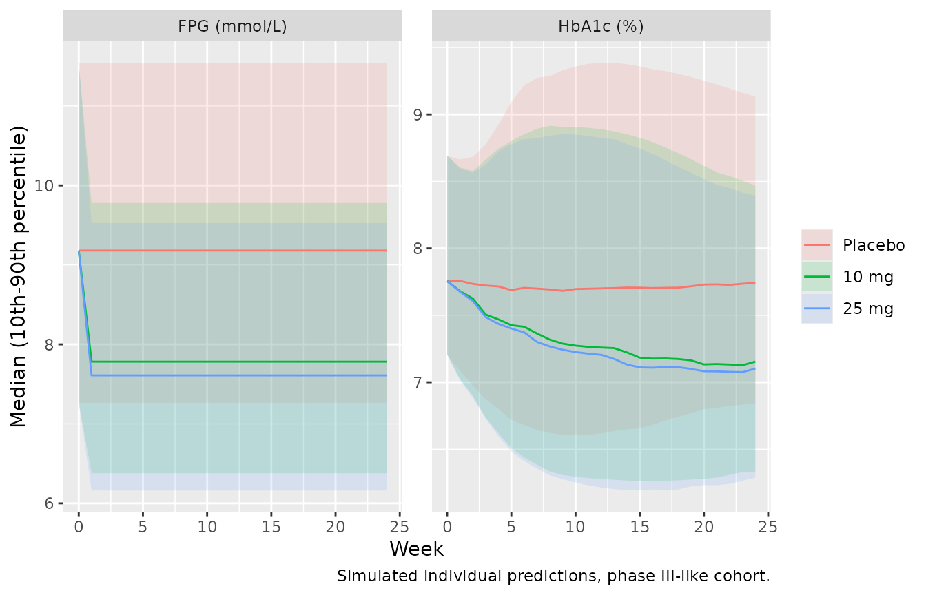
HbA1c and FPG over 24 weeks
sim |>
  dplyr::filter(time %% 168 == 0) |>
  dplyr::select(id, time, treatment, FPG_sim = glucose, HbA1c_sim = hba1c) |>
  tidyr::pivot_longer(c(FPG_sim, HbA1c_sim), names_to = "endpoint", values_to = "value") |>
  dplyr::mutate(endpoint = dplyr::recode(endpoint, FPG_sim = "FPG (mmol/L)", HbA1c_sim = "HbA1c (%)")) |>
  dplyr::group_by(endpoint, treatment, week = time / 168) |>
  dplyr::summarise(
    Q10 = quantile(value, 0.1), Q50 = median(value), Q90 = quantile(value, 0.9),
    .groups = "drop"
  ) |>
  ggplot(aes(week, Q50, colour = treatment, fill = treatment)) +
  geom_ribbon(aes(ymin = Q10, ymax = Q90), alpha = 0.15, colour = NA) +
  geom_line() +
  facet_wrap(~endpoint, scales = "free_y") +
  labs(
    x = "Week", y = "Median (10th-90th percentile)", colour = NULL, fill = NULL,
    caption = "Simulated individual predictions, phase III-like cohort."
  )
Replicate Table 1: change in HbA1c at week 24
Table 1 of Fayette 2023 gives the mean simulated change in HbA1c from baseline to week 24 per arm (design phase with phase II covariates; analysis phase with the target-trial covariates), the placebo-corrected means, and the observed phase III result.
chg <- sim |>
  dplyr::filter(time %in% c(0, 4032)) |>
  dplyr::select(id, treatment, time, hba1c) |>
  tidyr::pivot_wider(names_from = time, values_from = hba1c, names_prefix = "t") |>
  dplyr::mutate(d_hba1c = t4032 - t0)

arm_means <- chg |>
  dplyr::group_by(treatment) |>
  dplyr::summarise(baseline = mean(t0), change = mean(d_hba1c), .groups = "drop") |>
  dplyr::mutate(placebo_corrected = change - change[treatment == "Placebo"])

published <- tibble::tibble(
  treatment = factor(c("Placebo", "10 mg", "25 mg"), levels = levels(arms$treatment)),
  design_change = c(-0.055, -0.54, -0.61),
  design_pc = c(NA, -0.48, -0.56),
  analysis_change = c(-0.049, -0.55, -0.61),
  analysis_pc = c(NA, -0.50, -0.56),
  phase3_observed_pc = c(NA, -0.55, -0.69)
)

arm_means |>
  dplyr::left_join(published, by = "treatment") |>
  dplyr::rename(
    "Arm" = treatment,
    "Simulated baseline HbA1c (%)" = baseline,
    "Simulated change" = change,
    "Simulated placebo-corrected" = placebo_corrected,
    "Paper design-phase change" = design_change,
    "Paper design-phase placebo-corrected" = design_pc,
    "Paper analysis-phase change" = analysis_change,
    "Paper analysis-phase placebo-corrected" = analysis_pc,
    "Observed phase III placebo-corrected" = phase3_observed_pc
  ) |>
knitr::kable(digits = 3, caption = "Mean change in HbA1c (%) from baseline to week 24. Paper values from Fayette 2023 Table 1.")| Arm | Simulated baseline HbA1c (%) | Simulated change | Simulated placebo-corrected | Paper design-phase change | Paper design-phase placebo-corrected | Paper analysis-phase change | Paper analysis-phase placebo-corrected | Observed phase III placebo-corrected |
|---|---|---|---|---|---|---|---|---|
| Placebo | 7.874 | 0.010 | 0.000 | -0.055 | NA | -0.049 | NA | NA |
| 10 mg | 7.874 | -0.532 | -0.543 | -0.540 | -0.48 | -0.550 | -0.50 | -0.55 |
| 25 mg | 7.874 | -0.603 | -0.614 | -0.610 | -0.56 | -0.610 | -0.56 | -0.69 |
The placebo-corrected effect is the quantity the paper borrows on. A mis-transcribed GMAX, AUC50, HbA1c ratio or the uncentred baseline-FPG effect on HbA1c production moves it by tens of percent. The check below holds both the per-arm mean change and the placebo-corrected change within 0.1 percentage points of the paper’s analysis-phase values (simulated with the target-trial covariates, as here). A 2000-participant paired simulation of the same design gave -0.030, -0.555 and -0.622 for the three arms (placebo-corrected -0.525 and -0.593), so the expected differences are about 0.03 percentage points; the paper’s values also include parameter uncertainty, which this simulation does not.
ref <- published[match(arm_means$treatment, published$treatment), ]
arm_diff <- arm_means$change - ref$analysis_change
pc_diff <- (arm_means$placebo_corrected - ref$analysis_pc)[-1]
arm_diff
#> [1] 0.059493193 0.017595140 0.006540223
pc_diff
#> [1] -0.04289805 -0.05395297
stopifnot(all(abs(arm_diff) < 0.1), all(abs(pc_diff) < 0.1))
The typical participant (all random effects zero) has a larger placebo response, about -0.16 percentage points at week 24. The additive random effect on the placebo amplitude is wide (SD 0.66 around a typical 0.173), and HbA1c responds nonlinearly to it, so the population mean placebo response is much closer to zero than the typical-participant value. That is what Table 1 reports.
The mean simulated baseline HbA1c of 7.87% also matches the population: the trials enrolled adults with HbA1c between about 6.5% and 10% (Table S1 inclusion criteria). This supports reading the baseline-FPG effect on kHbA1c,in as uncentred (exp(0.04 * FPG)); with the covariate centred on a typical FPG, baseline HbA1c would be about 2.23 + 4.56 = 6.8%, below the inclusion range, and the drug effect about 30% smaller.
Steady-state check of the HbA1c model
Appendix S1 gives the eventual steady-state change in HbA1c, Delta HbA1c_ss = (kin/kout) * ((FPG_ss / FPG0)^power - 1), with FPG_ss = FPG0 / (1 + STIM). The typical-value model, solved for 5 years so the placebo term has decayed, must reproduce it.
mod_typ <- mod |> rxode2::zeroRe()
#> ℹ parameter labels from comments will be replaced by 'label()'
ss_cov <- data.frame(
  id = 1L, AGE = 50, BMI = 25, SEXF = 0, RACE_ASIAN = 0, SMOKE_NEVER = 0, SMOKE_CURRENT = 0,
  CRCL = 100, TPRO = 70, ALT = 20, AST = 20, ALP = 70, LDH = 160, FPG = 9.61
)
ss_check <- lapply(c(10, 25), function(d) {
  # The PD model sees the dose only through DOSE_EMPA_MGD (AUCss = dose / CL),
  # so no dosing records are needed for the FPG / HbA1c steady state.
  ev <- cbind(ss_cov, time = c(0, 43800), evid = 0L, amt = 0, cmt = "hba1c", DOSE_EMPA_MGD = d)
  s <- rxode2::rxSolve(mod_typ, events = ev, returnType = "data.frame")
  ui <- rxode2::rxode2(mod)
  th <- ui$theta
  cl <- exp(th[["lcl"]])
  auc <- 2217.8 * d / cl
  stim <- exp(th[["lemax"]]) * auc / (exp(th[["lauc50"]]) + auc)
  ratio <- exp(th[["lhba1c_ratio"]] + th[["e_fpg_hba1c_ratio"]] * 9.61)
  data.frame(
    dose_mg = d,
    simulated = s$hba1c[2] - s$hba1c[1],
    closed_form = ratio * ((1 / (1 + stim))^th[["gamma_hba1c"]] - 1)
  )
})
#> ℹ omega/sigma items treated as zero: 'etalcl', 'etalvp', 'etalka', 'etalrbase_glucose', 'etalemax', 'etapbo_hba1c', 'etalhba1c_ratio'
#> ℹ parameter labels from comments will be replaced by 'label()'
#> ℹ omega/sigma items treated as zero: 'etalcl', 'etalvp', 'etalka', 'etalrbase_glucose', 'etalemax', 'etapbo_hba1c', 'etalhba1c_ratio'
#> ℹ parameter labels from comments will be replaced by 'label()'
ss_check <- do.call(rbind, ss_check)
knitr::kable(ss_check, digits = 4, caption = "Typical subject: simulated 5-year change vs the Appendix S1 steady-state formula.")| dose_mg | simulated | closed_form |
|---|---|---|
| 10 | -0.4978 | -0.4978 |
| 25 | -0.5797 | -0.5797 |
PKNCA validation
The PD model is driven by AUCss = 2217.8 * DOSE / (CL/F) (Appendix S1). The steady-state AUC over the last dosing interval from the ODE solution is compared with that closed form for each simulated subject. Fayette 2023 reports no NCA table, so this is an internal consistency check of the PK model and the exposure driver; both sides use the same individual parameters.
sim_nca <- sim |>
  dplyr::filter(DOSE_EMPA_MGD > 0, time >= 4008, !is.na(Cc)) |>
  dplyr::mutate(time = time - 4008) |>
  dplyr::select(id, time, Cc, treatment) |>
  dplyr::mutate(treatment = droplevels(treatment))

dose_df <- sim_nca |>
  dplyr::distinct(id, treatment) |>
  dplyr::left_join(subjects |> dplyr::select(id, amt = DOSE_EMPA_MGD), by = "id") |>
  dplyr::mutate(time = 0)

conc_obj <- PKNCA::PKNCAconc(sim_nca, Cc ~ time | treatment + id)
dose_obj <- PKNCA::PKNCAdose(dose_df, amt ~ time | treatment + id)
intervals <- data.frame(start = 0, end = 24, cmax = TRUE, tmax = TRUE, auclast = TRUE, cmin = TRUE)
nca_res <- PKNCA::pk.nca(PKNCA::PKNCAdata(conc_obj, dose_obj, intervals = intervals))

nca_wide <- as.data.frame(nca_res$result) |>
  dplyr::select(id, treatment, PPTESTCD, PPORRES) |>
  tidyr::pivot_wider(names_from = PPTESTCD, values_from = PPORRES)

auc_chk <- nca_wide |>
  dplyr::left_join(sim |> dplyr::filter(time == 4008) |> dplyr::select(id, auc_ss), by = "id") |>
  dplyr::mutate(pct_diff = 100 * (auclast / auc_ss - 1))

auc_chk |>
  dplyr::group_by(treatment) |>
  dplyr::summarise(
    cmax = median(cmax), tmax = median(tmax), cmin = median(cmin),
    auclast = median(auclast), auc_ss = median(auc_ss),
    median_pct_diff = median(pct_diff), .groups = "drop"
  ) |>
  dplyr::rename(
    "Arm" = treatment,
    "Cmax,ss (nmol/L)" = cmax,
    "Tmax,ss (h)" = tmax,
    "Cmin,ss (nmol/L)" = cmin,
    "AUC0-24,ss PKNCA (nmol*h/L)" = auclast,
    "AUCss = 2217.8*Dose/CL (nmol*h/L)" = auc_ss,
    "Median % difference" = median_pct_diff
  ) |>
knitr::kable(digits = 2, caption = "Steady-state NCA (median over subjects) vs the model's exposure driver.")| Arm | Cmax,ss (nmol/L) | Tmax,ss (h) | Cmin,ss (nmol/L) | AUC0-24,ss PKNCA (nmol*h/L) | AUCss = 2217.8Dose/CL (nmolh/L) | Median % difference |
|---|---|---|---|---|---|---|
| 10 mg | 298.54 | 1.5 | 24.71 | 2170.18 | 2199.04 | -1 |
| 25 mg | 746.35 | 1.5 | 61.77 | 5425.46 | 5497.60 | -1 |
Assumptions and deviations
- Covariate centring values. Appendix S1 writes the covariate model as TVP = exp(theta + sum theta_l * cov_l). Taken literally with raw ages, BMIs and laboratory values this is meaningless for the PK model (an age coefficient of -0.305 would scale CL/F by exp(-0.305 * 58)), and the coefficients have the size and sign of the Baron 2016 power exponents. The continuous PK covariates are therefore implemented as power terms, (cov / ref)^theta. Fayette 2023 does not print the reference values; the maintainers used those of the predecessor model (Baron 2016 Table S1): age 50 years, BMI 25 kg/m^2 (20 kg/m^2 for V2/F), eGFR 100 mL/min/1.73 m^2, total protein 70 g/L, ALT 20, AST 20, AP 70 and LDH 160 U/L. The typical CL/F, V2/F, V3/F, Q/F and ka (11.5 L/h, 3.3 L, 75 L, 6.3 L/h and 0.196 1/h) agree with Baron 2016 to within about 10%, as expected for a refit of the same model.
- Baseline FPG effect on kHbA1c,in. KHINFPGB1 = 0.04 is implemented uncentred, exp(0.04 * FPG) with FPG in mmol/L, exactly as the printed covariate equation reads. This gives realistic baseline HbA1c values and reproduces the placebo-corrected effects of Table 1 (see above).
- FPG equation. Appendix S1 Eq. 1 prints the removal term as kFPGout * (1 + STIM) without the FPG state. The text calls kFPGout a first-order rate constant and sets kFPGin = BFPG * kFPGout for a baseline steady state, which only holds when removal is kFPGout * FPG * (1 + STIM); the model uses that form, as in Baron 2016.
- BFPG-GMAX random effects. Table S6 labels the off-diagonal element ‘Corr1 omega^2 BFPG,GMAX = 0.0519’. It is encoded as a covariance (a correlation of 0.45), consistent with the omega^2 notation and with the PK table, where omega^2 CL,V3 = 0.0277 is likewise a covariance.
- Placebo random effect. Table S6 reports the variance of the additive random effect on the placebo amplitude as 0.431, the same value as for GMAX (with a different RSE, 99.8% vs 10.9%). It is used as printed. The placebo term is applied from the first dose (time 0) onwards, with t in the exponential decay being time after the first dose.
- Placebo response. The typical-participant placebo response (-0.16 percentage points at week 24) is larger than the population mean in Table 1 (-0.049). The difference comes from the wide additive random effect on the placebo amplitude, and the simulated population mean reproduces the paper.
- PK residual error. Table S4 reports separate residual variances for studies 2-4-15 (intensive sampling, 0.0278) and studies 9-10 (sparse 12-week phase IIb sampling, 0.137). The model carries the studies 9-10 value; the reported CVs equal sqrt(exp(sigma^2) - 1), so the error is log-normal on the concentration. PK residual error does not affect the PD predictions.
- Black race. The Black-race coefficients in Table S4 are 0 with no standard error and are not part of the model.
- eGFR cap. eGFR values above 120 mL/min/1.73 m^2 are capped at 120 inside the model, as in the paper’s covariate analysis (Table S2 footnote).
- Virtual cohort. Laboratory covariates not tabulated in Table S2 are set to their reference values; observed baseline FPG is drawn log-normally (SD 0.2 on the log scale) around the model’s typical baseline FPG for the participant’s race group. Age, BMI and eGFR are drawn from normal distributions with the Table S2 means and SDs, truncated to plausible ranges.
- No erratum or correction notice for Fayette 2023 was found (checked 2026-10-27).