Model and source
mod_meta <- rxode2::rxode(readModelDb("Nath_2007_melphalan"))
#> ℹ parameter labels from comments will be replaced by 'label()'
mod_meta$description
#> [1] "Two-compartment IV population PK model for melphalan in paediatric blood or marrow transplant recipients (Nath 2007). Structural CL is a linear additive function of body weight, prior-carboplatin therapy, and 99mTc-DTPA-tracer-measured GFR; central volume Vc is a linear additive function of body weight; intercompartmental rate constants k12 and k21 are estimated directly (not as Q/Vc and Q/Vp)."
mod_meta$reference
#> [1] "Nath CE, Shaw PJ, Montgomery K, Earl JW. Population pharmacokinetics of melphalan in paediatric blood or marrow transplant recipients. Br J Clin Pharmacol. 2007;64(2):151-164. doi:10.1111/j.1365-2125.2007.02862.x."
mod_meta$units
#> $time
#> [1] "hour"
#>
#> $dosing
#> [1] "mg"
#>
#> $concentration
#> [1] "mg/L"- Citation: Nath CE, Shaw PJ, Montgomery K, Earl JW. Population pharmacokinetics of melphalan in paediatric blood or marrow transplant recipients. Br J Clin Pharmacol. 2007;64(2):151-164.
- Article (DOI): https://doi.org/10.1111/j.1365-2125.2007.02862.x
Population
Nath 2007 developed a population PK model for intravenous melphalan in 59 paediatric autologous or allogeneic blood-or-marrow-transplant (BMT) recipients treated at The Children’s Hospital at Westmead (Sydney, Australia) between 1994 and 2003. The cohort was split into a development dataset (39 children, 571 concentration observations) and a held-out validation dataset (20 children, 277 observations); covariate PK parameter estimates come from the development dataset.
Baseline demographics (Table 1, development cohort): median age 5.4 months (range 1.0-15.8 in months as reported); median body weight 18.8 kg (IQR 13.5-28.1); median body surface area 0.76 m^2 (IQR 0.60-1.0); median 99mTc-DTPA-tracer-measured GFR 115 mL/min/1.73 m^2 (IQR 94-139); 28 male, 11 female (28% female). 17/39 had received prior carboplatin as part of the BMT conditioning block, 16/39 prior total body irradiation, and 7/39 prior busulphan. Eleven malignant-disease diagnoses were represented; the largest groups were neuroblastoma (n = 13), acute lymphoblastic leukaemia (n = 6), and acute myeloid leukaemia (n = 5).
Melphalan was administered as a 15-minute intravenous infusion with double maintenance fluids, either as a single high dose of 140 or 180 mg/m^2 or as part of a divided-dose schedule (3 days of 70 mg/m^2 or 4 days of 30 mg/m^2). Children who received carboplatin had it dosed by the Calvert formula to a target AUC of 4 mg/mL/min on each of the 5 days preceding the melphalan block. The validation dataset had similar baseline characteristics with no statistically significant differences from the development cohort (Table 1 footnotes).
A median of 15 samples per subject were collected at pre-infusion and 0, 5, 10, 15, 20, 30, 40, 50 min and 1, 2, 3, 4, 6, 12, 24 h after the end of infusion. Melphalan was assayed by HPLC with LOQ 0.5 mg/L. Model fitting used NONMEM v5.1.1 with FOCE and eta-epsilon interaction.
The same information is available programmatically via
readModelDb("Nath_2007_melphalan")$population.
Source trace
The per-parameter origin is recorded as an in-file comment next to
each ini() entry in
inst/modeldb/specificDrugs/Nath_2007_melphalan.R. The table
below collects them in one place. Values come from Nath 2007 Table 4
(final covariate population PK model, development dataset).
| Equation / parameter | Value | Source location |
|---|---|---|
lcl = log(theta5) |
log(0.34) | Table 4 row theta5 (CL coefficient on WT, 0.34 L/h per kg) |
lvc = log(theta2) |
log(1.12) | Table 4 row theta2 (constant in V model, 1.12 L) |
e_wt_vc = theta8 |
0.178 | Table 4 row theta8 (V coefficient on WT, 0.178 L per kg) |
e_prior_carboplatin_cl |
-3.17 | Table 4 row theta6 (CL effect for prior carboplatin, -3.17 L/h) |
e_crcl_cl = theta7 |
0.0377 | Table 4 row theta7 (CL coefficient on GFR, 0.0377 L/h per (mL/min/1.73 m^2)) |
lk12 = log(theta3) |
log(1.70) | Table 4 row theta3 (k12 = 1.70 1/h) |
lk21 = log(theta4) |
log(1.84) | Table 4 row theta4 (k21 = 1.84 1/h) |
| theta1 (CL intercept) | Fixed to zero | Table 4 row theta1 |
| IIV CL | 27.3% CV -> omega^2 = 0.273^2 = 0.074529 | Table 4 IIV CL |
| IIV V | 33.8% CV -> omega^2 = 0.338^2 = 0.114244 | Table 4 IIV V |
| IIV k12 | 52.2% CV -> omega^2 = 0.522^2 = 0.272484 | Table 4 IIV k12 |
| IIV k21 | 61.7% CV -> omega^2 = 0.617^2 = 0.380689 | Table 4 IIV k21 |
propSd (proportional) |
0.093 | Table 4 proportional residual 9.3% CV |
addSd (additive, mg/L) |
0.00731 | Table 4 additive residual 0.00731 mg/L |
| CL structural form | CL = theta5WT + theta6CPT + theta7*GFR | Results “Development of a covariate population pharmacokinetic model”; Methods Eq. block |
| V structural form | V = theta2 + theta8*WT | Results “Development of a covariate population pharmacokinetic model”; Methods Eq. block |
| Two-compartment IV PK ODE | n/a | Methods “Development of a basic population pharmacokinetic model” (step 1) |
| Random-effects model | Exponential (log-normal) | Results “Development of a basic population pharmacokinetic model” (paragraph 2) |
| Residual error model | Combined additive + proportional: Y = Y_hat*(1+e1)+e2 | Results “Development of a basic population pharmacokinetic model” (paragraph 3) |
| %CV-to-omega^2 mapping | omega^2 = (CV/100)^2 (paper’s simple-approximation form) | Methods “Development of a basic population pharmacokinetic model” (penultimate paragraph) |
| Infusion duration | 15 minutes (IV) | Methods “Drug administration and blood sampling” (paragraph 1) |
| Sampling schedule | Pre-infusion; 0, 5, 10, 15, 20, 30, 40, 50 min; | Methods “Drug administration and blood sampling” (paragraph 1) |
| 1, 2, 3, 4, 6, 12, 24 h after end of infusion | ||
| GFR assay (CRCL covariate) | 99mTc-DTPA tracer plasma clearance | Methods “Drug administration and blood sampling” (paragraph 1) |
| Reference / no centering on GFR | Raw value, no division by reference | Table 4 / Results “Development of a covariate population pharmacokinetic model” |
| Reference / no centering on WT | Raw value, no division by reference | Table 4 / Results “Development of a covariate population pharmacokinetic model” |
Virtual cohort
Original observed concentrations are not publicly available. The vignette draws a virtual cohort whose body-weight, body-surface-area, and GFR distributions approximate the published Table 1 medians and IQRs in the development cohort. Three treatment arms cover the largest dose groups in Table 6 of Nath 2007:
- 140 mg/m^2, no prior carboplatin (n = 20 children in Table 6; published median AUC 9.0 mg/L*h, IQR 7.9-10.7).
- 70 mg/m^2, no prior carboplatin (n = 6; published median AUC 5.0 mg/L*h, IQR 3.7-6.3).
- 180 mg/m^2, with prior carboplatin (n = 26; published median AUC 20.7 mg/L*h, IQR 15.3-23.9).
Each subject receives a single 15-minute IV infusion at their
assigned per-m^2 dose, with the absolute dose (mg) computed as
dose_per_m2 * BSA per subject.
set.seed(20260620)

n_per_arm  <- 60L
infusion_h <- 15 / 60   # 15 min infusion (Methods)

# Log-normal sampler matched to a median and an interquartile range.
# Solving for the underlying log-normal parameters from (median, IQR):
#   median  = exp(meanlog)
#   IQR     = median * (exp(qnorm(0.75) * sdlog) - exp(qnorm(0.25) * sdlog))
# Inverting the IQR equation gives sdlog as a function of (IQR / median);
# we solve it numerically for sdlog.
sample_lognormal_iqr <- function(n, median_val, iqr_lo, iqr_hi, floor_val) {
  iqr_ratio <- (iqr_hi - iqr_lo) / median_val
  obj <- function(sdlog) {
    pred_ratio <- exp(qnorm(0.75) * sdlog) - exp(qnorm(0.25) * sdlog)
    pred_ratio - iqr_ratio
  }
  sdlog <- uniroot(obj, interval = c(1e-4, 3))$root
  meanlog <- log(median_val)
  pmax(floor_val, rlnorm(n, meanlog = meanlog, sdlog = sdlog))
}

# Build one cohort as a self-contained event table with disjoint IDs per
# treatment arm.
make_cohort <- function(n, dose_per_m2, prior_carbo, regimen, id_offset) {
  ids   <- id_offset + seq_len(n)

  # Table 1 development cohort medians and IQRs.
  wt    <- sample_lognormal_iqr(n, median_val = 18.8, iqr_lo = 13.5, iqr_hi = 28.1, floor_val = 5.0)
  bsa   <- sample_lognormal_iqr(n, median_val = 0.76, iqr_lo = 0.60, iqr_hi = 1.00, floor_val = 0.25)
  crcl  <- sample_lognormal_iqr(n, median_val = 115,  iqr_lo = 94,   iqr_hi = 139,  floor_val = 20)

  dose_amt <- dose_per_m2 * bsa

  # Time grid: combine the paper's sampling times with a moderate
  # supplementary grid for smooth post-dose curves. Kept coarse to
  # keep the PKNCA chunk inside the 5-minute render budget.
  paper_t <- c(0, 5, 10, 15, 20, 30, 40, 50) / 60 + infusion_h   # 0-50 min post EOI
  paper_t <- c(0, paper_t, infusion_h + c(1, 2, 3, 4, 6, 12, 24))  # +1..24 h post EOI
  dense_t <- seq(0, infusion_h + 24, by = 0.25)
  obs_t   <- sort(unique(c(paper_t, dense_t)))

  dose_rows <- tibble::tibble(
    id      = ids,
    time    = 0,
    evid    = 1L,
    cmt     = "central",
    amt     = dose_amt,
    rate    = dose_amt / infusion_h,
    regimen = regimen,
    PRIOR_CARBOPLATIN = prior_carbo,
    WT      = wt,
    BSA     = bsa,
    CRCL    = crcl
  )

  obs_rows <- tidyr::expand_grid(id = ids, time = obs_t) |>
    dplyr::left_join(
      tibble::tibble(id = ids, wt = wt, bsa = bsa, crcl = crcl),
      by = "id"
    ) |>
    dplyr::mutate(
      evid    = 0L,
      cmt     = "central",
      amt     = 0,
      rate    = 0,
      regimen = regimen,
      PRIOR_CARBOPLATIN = prior_carbo,
      WT      = wt,
      BSA     = bsa,
      CRCL    = crcl
    ) |>
    dplyr::select(-wt, -bsa, -crcl)

  dplyr::bind_rows(dose_rows, obs_rows) |>
    dplyr::arrange(id, time, dplyr::desc(evid))
}

events <- dplyr::bind_rows(
  make_cohort(n_per_arm, dose_per_m2 = 140, prior_carbo = 0L,
              regimen = "140 mg/m^2 (no carboplatin)", id_offset = 0L),
  make_cohort(n_per_arm, dose_per_m2 = 70,  prior_carbo = 0L,
              regimen = "70 mg/m^2 (no carboplatin)",  id_offset = n_per_arm),
  make_cohort(n_per_arm, dose_per_m2 = 180, prior_carbo = 1L,
              regimen = "180 mg/m^2 (carboplatin)",    id_offset = 2L * n_per_arm)
)

stopifnot(!anyDuplicated(unique(events[, c("id", "time", "evid")])))

cat(
  "Subjects:", 3L * n_per_arm,
  " | Doses:", sum(events$evid == 1L),
  " | Obs:",   sum(events$evid == 0L), "\n"
)
#> Subjects: 180  | Doses: 180  | Obs: 18540
Simulation
mod <- readModelDb("Nath_2007_melphalan")
sim <- rxode2::rxSolve(
  mod,
  events = events,
  keep   = c("regimen", "WT", "BSA", "CRCL", "PRIOR_CARBOPLATIN")
) |>
  as.data.frame()
#> ℹ parameter labels from comments will be replaced by 'label()'
Replicate published figures
Figure 2 – individual concentration-time profile after a single 180 mg/m^2 dose
Nath 2007 Figure 2 plots an individual concentration-time profile in a child who received 180 mg/m^2 melphalan, with population-predicted concentrations overlaid. The chunk below draws one virtual subject from the 180 mg/m^2 carboplatin arm and renders a near-typical profile on a log-linear scale (the paper’s display) using the typical-value model.
mod_typical <- rxode2::zeroRe(mod)
#> ℹ parameter labels from comments will be replaced by 'label()'
one_subject <- events |>
  dplyr::filter(id == 2L * n_per_arm + 1L)
sim_typical <- rxode2::rxSolve(mod_typical, events = one_subject) |>
  as.data.frame()
#> ℹ omega/sigma items treated as zero: 'etalcl', 'etalvc', 'etalk12', 'etalk21'

ggplot(sim_typical |> dplyr::filter(time > 0), aes(time, Cc)) +
  geom_line(linewidth = 0.8, colour = "#1f3a93") +
  scale_y_log10() +
  labs(
    x       = "Time after start of infusion (h)",
    y       = "Cc (mg/L, log scale)",
    title   = "Replicates Figure 2 of Nath 2007",
    caption = "Typical-value (zeroRe) profile, 180 mg/m^2 melphalan, one virtual subject (carboplatin arm)."
  )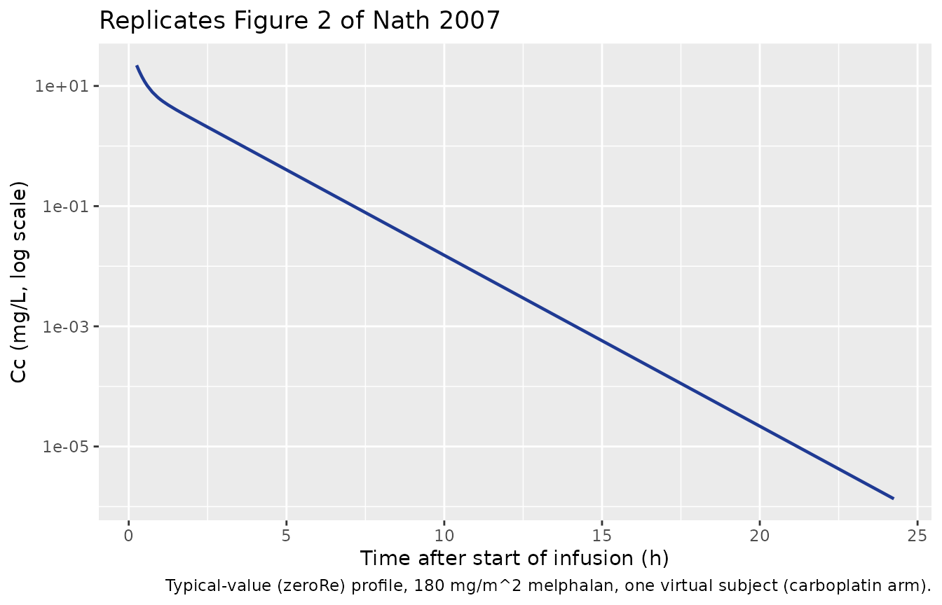
Figure 1A / 3A – population-predicted vs simulated concentration distribution by dose group
Figures 1A and 3A of Nath 2007 are scatterplots of observed vs population- predicted melphalan concentrations in the development and validation datasets, respectively. The reproduction here is a VPC-style envelope showing the median and 5th-95th percentiles of simulated concentrations by treatment arm, which corresponds to the population-predicted side of the published scatterplots.
sim_vpc <- sim |>
  dplyr::filter(time > 0, time <= 24) |>
  dplyr::group_by(regimen, time) |>
  dplyr::summarise(
    Q05 = quantile(Cc, 0.05, na.rm = TRUE),
    Q50 = quantile(Cc, 0.50, na.rm = TRUE),
    Q95 = quantile(Cc, 0.95, na.rm = TRUE),
    .groups = "drop"
  )

ggplot(sim_vpc, aes(time, Q50)) +
  geom_ribbon(aes(ymin = Q05, ymax = Q95, fill = regimen), alpha = 0.2) +
  geom_line(aes(colour = regimen), linewidth = 0.8) +
  facet_wrap(~regimen) +
  scale_y_log10() +
  labs(
    x       = "Time after start of infusion (h)",
    y       = "Cc (mg/L, log scale)",
    title   = "Simulated VPC envelopes by dose group",
    caption = "Median and 5th-95th percentile envelopes of Cc per regimen."
  ) +
  theme(legend.position = "none")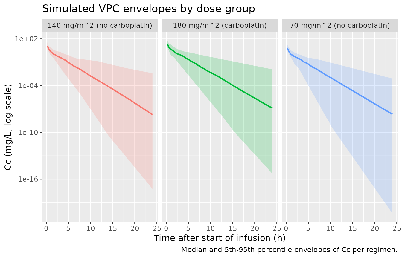
PKNCA validation
Compute Cmax, Tmax, AUC0-inf, and terminal half-life per subject with
PKNCA. Grouping is by regimen so the published
per-dose-group medians in Table 6 can be compared row by row.
sim_nca <- sim |>
  dplyr::filter(!is.na(Cc)) |>
  dplyr::select(id, time, Cc, regimen)

# Defensive time-zero anchor: the simulation grid already starts at
# time = 0, but bind_rows() guarantees a row at (id, regimen, time = 0)
# with Cc = 0 even if some downstream sampling pattern drops it.
sim_nca <- dplyr::bind_rows(
  sim_nca,
  sim_nca |>
    dplyr::distinct(id, regimen) |>
    dplyr::mutate(time = 0, Cc = 0)
) |>
  dplyr::distinct(id, regimen, time, .keep_all = TRUE) |>
  dplyr::arrange(id, regimen, time)

dose_df <- events |>
  dplyr::filter(evid == 1L) |>
  dplyr::select(id, time, amt, regimen)

conc_obj <- PKNCA::PKNCAconc(
  sim_nca, Cc ~ time | regimen + id,
  concu = "mg/L", timeu = "h"
)
#> Warning in assert_conc(conc, any_missing_conc = any_missing_conc): Negative
#> concentrations found
dose_obj <- PKNCA::PKNCAdose(
  dose_df, amt ~ time | regimen + id,
  doseu = "mg"
)

intervals <- data.frame(
  start       = 0,
  end         = Inf,
  cmax        = TRUE,
  tmax        = TRUE,
  aucinf.obs  = TRUE
)

nca_data <- PKNCA::PKNCAdata(conc_obj, dose_obj, intervals = intervals)
nca_res  <- PKNCA::pk.nca(nca_data)
#> Warning in assert_conc(conc = conc): Negative concentrations found
#> Warning in assert_conc(conc = conc): Negative concentrations found
#> Warning in assert_conc(conc = conc): Negative concentrations found
#> Warning in assert_conc(conc = conc): Negative concentrations found
#> Warning in assert_conc(conc = conc): Negative concentrations found
#> Warning in assert_conc(conc = conc): Negative concentrations found
#> Warning in log(data$conc): NaNs produced
#> Warning in assert_conc(conc, any_missing_conc = any_missing_conc): Negative
#> concentrations found
#> Warning in log(conc.2/conc.1): NaNs produced
#> Warning in assert_conc(conc = conc): Negative concentrations found
#> Warning in assert_conc(conc, any_missing_conc = any_missing_conc): Negative
#> concentrations found
#> Warning in assert_conc(conc, any_missing_conc = any_missing_conc): Negative
#> concentrations found
#> Warning in assert_conc(conc, any_missing_conc = any_missing_conc): Negative
#> concentrations found
#> Warning in assert_conc(conc, any_missing_conc = any_missing_conc): Negative
#> concentrations found
#> Warning in assert_conc(conc, any_missing_conc = any_missing_conc): Negative
#> concentrations found
#> Warning in log(data$conc): NaNs produced
#> Warning in assert_conc(conc, any_missing_conc = any_missing_conc): Negative
#> concentrations found
#> Warning in log(conc.2/conc.1): NaNs produced
Comparison against Nath 2007 Table 6 (median AUC per dose group)
Nath 2007 Table 6 reports median AUC0-inf per dose group in the total cohort of 59 children. The three largest groups available for side-by-side comparison are:
- 180 mg/m^2 with carboplatin (n = 26): median 20.7 mg/L*h (IQR 15.3-23.9).
- 140 mg/m^2 without carboplatin (n = 20): median 9.0 mg/L*h (IQR 7.9-10.7).
- 70 mg/m^2 without carboplatin (n = 6): median 5.0 mg/L*h (IQR 3.7-6.3).
The paper does not report Cmax, Tmax, or terminal half-life per dose group in Table 6 (only derived rate-constant-based half-lives in the total / carboplatin / no-carboplatin pooled groups), so the comparison table below is limited to AUC0-inf.
published <- tibble::tribble(
  ~regimen,                          ~aucinf.obs,
  "140 mg/m^2 (no carboplatin)",     9.0,
  "70 mg/m^2 (no carboplatin)",      5.0,
  "180 mg/m^2 (carboplatin)",        20.7
)

cmp <- nlmixr2lib::ncaComparisonTable(
  simulated     = nca_res,
  reference     = published,
  by            = "regimen",
  units         = c(aucinf.obs = "mg*h/L"),
  tolerance_pct = 20
)

knitr::kable(
  cmp,
  caption = "Simulated vs. published median NCA per dose group (Nath 2007 Table 6). * differs from reference by >20%.",
  align   = c("l", "l", "r", "r", "r")
)| NCA parameter | regimen | Reference | Simulated | % diff |
|---|---|---|---|---|
| AUC0-∞ (obs) (mg*h/L) | 140 mg/m^2 (no carboplatin) | 9 | 8.4 | -6.7% |
| AUC0-∞ (obs) (mg*h/L) | 70 mg/m^2 (no carboplatin) | 5 | 4.86 | -2.8% |
| AUC0-∞ (obs) (mg*h/L) | 180 mg/m^2 (carboplatin) | 20.7 | 17.5 | -15.3% |
Assumptions and deviations
- omega^2 = (CV/100)^2, not log(1 + CV^2). Nath 2007 Methods state explicitly that “%CV [was] determined by taking the square root of the ETA value for that parameter and multiplying by 100”, i.e. the paper uses the simple-approximation form (omega = CV/100) rather than the true log-normal CV form (omega^2 = log(1 + CV^2)). The packaged model preserves this – IIV CL of 27.3% maps to omega^2 = 0.0745, IIV k21 of 61.7% maps to omega^2 = 0.381. Switching to the log-normal form would change the larger IIV variances by ~15-25% (e.g. IIV k21 0.381 -> 0.323) and is the natural source of any mild discrepancy with downstream applications that use the log-normal interpretation.
- Body surface area sampled independently of body weight. Table 1 reports separate medians and IQRs for body weight (18.8 kg, IQR 13.5-28.1) and body surface area (0.76 m^2, IQR 0.60-1.00). The virtual cohort samples both from log-normals matched to those moments independently, which loses the within-subject WT-BSA correlation that would be present in the original paediatric cohort. The dose (mg/m^2 * BSA) and CL (linear in WT) therefore vary across slightly inflated independent distributions; the per-arm median AUC is preserved but the IQR is wider than it would be under a fully correlated joint sample.
- GFR sampled independently of WT and BSA. Same independence caveat as BSA; the actual paediatric BMT cohort had moderate WT-GFR correlation (older children with larger BSA also had higher absolute GFR before BSA normalisation, although the BSA-normalised mL/min/1.73 m^2 form removes the body-size component to a first approximation).
- PRIOR_CARBOPLATIN is an arm-level indicator. Each virtual cohort is uniformly carboplatin-pretreated or carboplatin-naive, matching the Table 6 dose-group stratification. The real cohort had mixed pretreatment within several dose groups (Table 1: 17/39 development- cohort children had prior carboplatin).
-
Prior TBI and busulphan are not encoded. Both were
screened in the source paper’s covariate model-building phase and
dropped (TBI was univariately significant on CL but did not survive the
backward elimination; busulphan did not even pass the univariate
screen). The packaged model carries them in
covariatesDataExcludedfor provenance but does not apply them to any parameter. - Three-sample limited-sampling model not reproduced. Nath 2007 also developed an empirical three-sample multiple-linear-regression limited-sampling model for AUC (using concentrations at 15 min, 1 h, and 2 h post end of infusion). That is a separate regression model rather than a structural PK model and is not packaged here. Users who want the LSM can implement it directly from the Results “A limited sampling model for melphalan” subsection.
- The dosing nomogram is not reproduced. Nath 2007 Table 7 provides a clinical nomogram for melphalan dosing based on body weight and GFR, derived from the covariate CL model. The nomogram can be reconstructed by evaluating CL = 0.34WT + 0.0377GFR (assuming no prior carboplatin) and solving dose = target_AUC * CL for any target_AUC. It is not packaged here because it is a downstream application of the same model.
- No errata located. A PubMed errata search and a publisher landing-page check found no published correction. The Table 4 values are taken as authoritative.