Vancomycin on CRRT (Hirunsomboon 2026)
Source:vignettes/articles/Hirunsomboon_2026_vancomycin.Rmd
Hirunsomboon_2026_vancomycin.RmdModel and source
- Citation: Hirunsomboon C, Pathumarak A, Nosoongnoen W, Tharanon V, Sukkha S. Population Pharmacokinetics of Vancomycin in Critically Ill Patients Undergoing Continuous Renal Replacement Therapy: Influence of Adsorptive Membranes. Clin Transl Sci. 2026;19:e70511. doi:10.1111/cts.70511
- Description: One-compartment population PK model for intravenous vancomycin in critically ill adults with acute kidney injury on continuous renal replacement therapy (CVVHDF), with an uncentered log-linear age effect and an adsorptive-membrane (oXiris) effect on clearance (Hirunsomboon 2026).
- Article: https://doi.org/10.1111/cts.70511 (open access, PMC12928122)
Hirunsomboon and colleagues fitted a population pharmacokinetic model of intravenous vancomycin in critically ill adults with acute kidney injury treated with continuous venovenous hemodiafiltration (CVVHDF). The question the study was built to answer is whether the adsorptive oXiris hemofilter – an AN69ST-derived membrane designed to bind cytokines and endotoxin – changes vancomycin clearance. A one-compartment model with first-order elimination, log-normal between-subject variability on CL and V, and a proportional residual error was selected (Table 2). Clearance falls with age and rises by about 5% with the oXiris membrane; no covariate was retained on V.
Population
Fifty-five adults admitted to the intensive care units of Ramathibodi Hospital, Bangkok, between 2014 and 2024 contributed 126 vancomycin concentrations from routine therapeutic drug monitoring (Results 3.1; Figure S1). Mean age was 61.5 +/- 16.0 years, 54.5% were male, and mean body weight was 60.5 +/- 17.3 kg. Mean SOFA score was 15.6, serum albumin 25.8 g/L, residual urine output 157 mL/day, and CRRT effluent flow 1.99 L/h (33.2 mL/kg/h). Twenty-six patients (47.3%) were treated with the oXiris membrane and the rest with a non-adsorptive membrane such as AN69. Every patient received a loading dose (mean 1362 mg) followed by a mean maintenance dose of 1122 mg/day (Table 1). Patients with end-stage renal disease were excluded.
pop <- readModelDb("Hirunsomboon_2026_vancomycin")()$population
str(pop[c("species", "n_subjects", "age_median", "weight_median", "dose_range")])
#> List of 5
#>  $ species      : chr "human"
#>  $ n_subjects   : int 55
#>  $ age_median   : chr "61.51 years (mean, SD 16.01)"
#>  $ weight_median: chr "60.49 kg (mean, SD 17.33)"
#>  $ dose_range   : chr "All patients received a loading dose (mean 1361.81 +/- 377.36 mg) followed by a maintenance dose of 1121.82 +/-"| __truncated__
Source trace
Every ini() value carries an in-file comment naming its
source. They are collected here for review.
| Equation / parameter | Value | Source location |
|---|---|---|
lcl (CL intercept at AGE = 0, non-adsorptive
membrane) |
2.82 L/h | Table 3, CL pop, RSE 19.0% |
lvc (V) |
94.97 L | Table 3, V pop, RSE 10.5% |
e_age_cl |
-0.007 1/year | Table 3, theta CL,age, RSE 44.0% |
e_filt_adsorptive_cl |
0.053 | Table 3, theta CL,MM=1, RSE 49.5% |
etalcl |
var = 0.2001^2 | Table 3, IIV CL (%) = 20.01, RSE 22.4% (omega x 100;
bootstrap median 0.17) |
etalvc |
var = 0.2163^2 | Table 3, IIV V (%) = 21.63, RSE 46.6% (omega x 100;
bootstrap median 0.19) |
propSd |
0.26 | Table 3, sigma (%) = 0.26, RSE 8.60% (bootstrap median
0.26) |
CL = 2.82 * exp(-0.007 * Age + 0.053 * MM) |
n/a | Results 3.2, displayed final clearance equation (‘use = 1, not use = 0’) |
| One compartment, first-order elimination | n/a | Results 3.2 and Table 2 |
| Log-normal IIV on CL and V, proportional residual error | n/a | Methods 2.3, Results 3.2 |
| No covariate on V | n/a | Results 3.2; Table S2 |
| Simulated regimens, 2 h infusions, AUC 48-72 h | n/a | Methods 2.4 |
| Published PTA values | n/a | Tables S3 (AUC/MIC > 400) and S4 (AUC/MIC > 600); Figure 4 |
mod <- readModelDb("Hirunsomboon_2026_vancomycin")
mod_typ <- rxode2::zeroRe(rxode2::rxode2(mod))
#> ℹ parameter labels from comments will be replaced by 'label()'
The age effect is uncentered
The Abstract and Discussion call 2.82 L/h “the population clearance”
and compare it with other CRRT studies (2.5 L/h, 2.53 L/h, 2.27 L/h).
But the displayed final equation enters age uncentered, so 2.82 L/h is
the clearance at AGE = 0. At the simulation age of 60 years
it is 2.82 * exp(-0.42) = 1.85 L/h.
The paper’s own Monte Carlo results decide between the two readings. Tables S3 and S4 report, for each regimen and MIC, the probability that AUC(48-72 h)/MIC exceeds 400 or 600 mg*h/L in a 60-year-old. A probability near 100% means the typical AUC/MIC sits above the threshold; a probability near 0% means it sits below. Each cell is therefore a bracket on the typical-value AUC(48-72 h), which we compute below from a typical-value solve of both readings with PKNCA.
regimens <- tibble::tribble(
  ~regimen,              ~ld, ~md,
  "1 g LD, 500 mg q24h", 1000,  500,
  "1.5 g LD, 750 mg q24h", 1500,  750,
  "2 g LD, 1 g q24h",    2000, 1000,
  "3 g LD, 1.5 g q24h",  3000, 1500
)
grid_typ <- tidyr::expand_grid(regimens, FILT_ADSORPTIVE = 0:1) |>
  mutate(id = dplyr::row_number(), AGE = 60)

# Doses at 0 h (loading) and 24, 48, 72 h (maintenance), each a 2 h infusion
# (Methods 2.4); the 72 h dose does not contribute to AUC(48-72 h).
make_events <- function(grid, obs_times) {
  doses <- grid |>
    tidyr::expand_grid(time = c(0, 24, 48, 72)) |>
    mutate(amt = ifelse(time == 0, ld, md), rate = amt / 2, evid = 1L)
  obs <- grid |>
    tidyr::expand_grid(time = obs_times) |>
    mutate(amt = 0, rate = 0, evid = 0L)
  bind_rows(doses, obs) |>
    mutate(cmt = "central") |>
    arrange(id, time, desc(evid)) |>
    select(id, time, amt, rate, evid, cmt, AGE, FILT_ADSORPTIVE)
}
ev_typ <- make_events(grid_typ, sort(unique(c(seq(0, 96, by = 0.25)))))

sim_typ <- rxode2::rxSolve(mod_typ, events = ev_typ, rtol = 1e-10, atol = 1e-12) |>
  as.data.frame() |>
  select(id, time, Cc) |>
  left_join(grid_typ |> select(id, regimen, ld, md, FILT_ADSORPTIVE), by = "id")
#> ℹ omega/sigma items treated as zero: 'etalcl', 'etalvc'
#> Warning: multi-subject simulation without without 'omega'
stopifnot(length(unique(sim_typ$id)) == nrow(grid_typ))
dose_typ <- ev_typ |>
  filter(evid == 1) |>
  left_join(grid_typ |> select(id, regimen), by = "id")
conc_typ <- PKNCA::PKNCAconc(sim_typ |> filter(!is.na(Cc)), Cc ~ time | regimen + FILT_ADSORPTIVE + id)
dose_obj <- PKNCA::PKNCAdose(dose_typ, amt ~ time | regimen + FILT_ADSORPTIVE + id)
nca_typ <- PKNCA::pk.nca(PKNCA::PKNCAdata(
  conc_typ, dose_obj,
  intervals = data.frame(start = 48, end = 72, auclast = TRUE)
))
auc_typ <- as.data.frame(nca_typ) |>
  filter(PPTESTCD == "auclast") |>
  select(regimen, FILT_ADSORPTIVE, auc = PPORRES)

# Closed-form AUC(48-72 h) for a one-compartment model with 2 h infusions,
# used to check the PKNCA trapezoid and to evaluate the centered reading.
auc_closed <- function(ld, md, cl, v = 94.97, tinf = 2) {
  k <- cl / v
  dt <- c(0, 24, 48)
  amt <- c(ld, md, md)
  conc <- function(t) {
    vapply(t, function(tt) {
      td <- tt - dt
      r <- amt / tinf
      sum(ifelse(td <= 0, 0,
        ifelse(td <= tinf, r / cl * (1 - exp(-k * td)),
          r / cl * (1 - exp(-k * tinf)) * exp(-k * (td - tinf))
        )
      ))
    }, numeric(1))
  }
  stats::integrate(conc, 48, 72, subdivisions = 1000L)$value
}
auc_typ <- auc_typ |>
  left_join(regimens, by = "regimen") |>
  mutate(
    cl_uncentered = 2.82 * exp(-0.007 * 60 + 0.053 * FILT_ADSORPTIVE),
    cl_centered = 2.82 * exp(0.053 * FILT_ADSORPTIVE),
    auc_uncentered_closed = mapply(auc_closed, ld, md, cl_uncentered),
    auc_centered_closed = mapply(auc_closed, ld, md, cl_centered)
  )
# The 0.25 h trapezoid over a smooth 24 h decline agrees with the closed form
# to ~1e-5 relative; 1e-3 still catches a wrong dose, rate or volume.
stopifnot(
  nrow(auc_typ) == 8L,
  max(abs(auc_typ$auc / auc_typ$auc_uncentered_closed - 1)) < 1e-3
)
The published PTA cells, transcribed from Tables S3 and S4. In Table S3 the two PTA columns are unlabelled; the first is taken as “with oXiris” because it is the lower of the two wherever they differ (higher clearance, lower AUC), which matches the labelled column order of Table S4.
pta_pub <- tibble::tribble(
  ~regimen, ~mic, ~target, ~pta_mm1, ~pta_mm0,
  "1 g LD, 500 mg q24h", 0.25, 400, 100, 100,
  "1 g LD, 500 mg q24h", 0.5, 400, 96.1, 100,
  "1 g LD, 500 mg q24h", 1, 400, 0, 0,
  "1 g LD, 500 mg q24h", 2, 400, 0, 0,
  "1 g LD, 500 mg q24h", 4, 400, 0, 0,
  "1.5 g LD, 750 mg q24h", 0.25, 400, 100, 100,
  "1.5 g LD, 750 mg q24h", 0.5, 400, 100, 100,
  "1.5 g LD, 750 mg q24h", 1, 400, 0, 6.48,
  "1.5 g LD, 750 mg q24h", 2, 400, 0, 0,
  "1.5 g LD, 750 mg q24h", 4, 400, 0, 0,
  "2 g LD, 1 g q24h", 0.25, 400, 100, 100,
  "2 g LD, 1 g q24h", 0.5, 400, 100, 100,
  "2 g LD, 1 g q24h", 1, 400, 96.1, 97.77,
  "2 g LD, 1 g q24h", 2, 400, 0, 0,
  "2 g LD, 1 g q24h", 4, 400, 0, 0,
  "3 g LD, 1.5 g q24h", 0.25, 400, 100, 100,
  "3 g LD, 1.5 g q24h", 0.5, 400, 100, 100,
  "3 g LD, 1.5 g q24h", 1, 400, 100, 100,
  "3 g LD, 1.5 g q24h", 2, 400, 0, 6.48,
  "3 g LD, 1.5 g q24h", 4, 400, 0, 0,
  "1 g LD, 500 mg q24h", 0.25, 600, 100, 100,
  "1 g LD, 500 mg q24h", 0.5, 600, 0, 97.8,
  "1 g LD, 500 mg q24h", 1, 600, 0, 0,
  "1 g LD, 500 mg q24h", 2, 600, 0, 0,
  "1 g LD, 500 mg q24h", 4, 600, 0, 0,
  "1.5 g LD, 750 mg q24h", 0.25, 600, 100, 100,
  "1.5 g LD, 750 mg q24h", 0.5, 600, 96.0, 97.8,
  "1.5 g LD, 750 mg q24h", 1, 600, 0, 0,
  "1.5 g LD, 750 mg q24h", 2, 600, 0, 0,
  "1.5 g LD, 750 mg q24h", 4, 600, 0, 0,
  "2 g LD, 1 g q24h", 0.25, 600, 100, 100,
  "2 g LD, 1 g q24h", 0.5, 600, 100, 100,
  "2 g LD, 1 g q24h", 1, 600, 0, 0,
  "2 g LD, 1 g q24h", 2, 600, 0, 0,
  "2 g LD, 1 g q24h", 4, 600, 0, 0,
  "3 g LD, 1.5 g q24h", 0.25, 600, 100, 100,
  "3 g LD, 1.5 g q24h", 0.5, 600, 100, 100,
  "3 g LD, 1.5 g q24h", 1, 600, 96.0, 97.8,
  "3 g LD, 1.5 g q24h", 2, 600, 0, 0,
  "3 g LD, 1.5 g q24h", 4, 600, 0, 0
) |>
  tidyr::pivot_longer(c(pta_mm1, pta_mm0), names_to = "arm", values_to = "pta_pub") |>
  mutate(FILT_ADSORPTIVE = ifelse(arm == "pta_mm1", 1L, 0L)) |>
  select(-arm)
stopifnot(nrow(pta_pub) == 80L, all(pta_pub$regimen %in% regimens$regimen))
A cell at or above 90% says the typical AUC/MIC is above the target; a cell at or below 10% says it is below. Every one of the 80 cells is one of the two.
bracket <- pta_pub |>
  left_join(auc_typ |> select(regimen, FILT_ADSORPTIVE, auc, auc_centered_closed),
    by = c("regimen", "FILT_ADSORPTIVE")
  ) |>
  mutate(
    pub_above = pta_pub >= 90,
    uncentered_ok = (auc / mic > target) == pub_above,
    centered_ok = (auc_centered_closed / mic > target) == pub_above
  )
stopifnot(
  nrow(bracket) == 80L,
  !anyNA(bracket$auc),
  all(bracket$pta_pub >= 90 | bracket$pta_pub <= 10)
)

bracket |>
  group_by(target) |>
  summarise(
    cells = n(),
    `consistent, uncentered age` = sum(uncentered_ok),
    `consistent, centered age` = sum(centered_ok)
  ) |>
  dplyr::rename("AUC/MIC target" = target, "Published cells" = cells) |>
knitr::kable()| AUC/MIC target | Published cells | consistent, uncentered age | consistent, centered age |
|---|---|---|---|
| 400 | 40 | 40 | 36 |
| 600 | 40 | 39 | 35 |
The uncentered (printed) equation is consistent with 79 of the 80 published cells; a centered reading, in which 2.82 L/h would be the clearance of a 60-year-old, is consistent with 71. The cells the centered reading gets wrong include the paper’s headline result: it puts the typical AUC/MIC of the recommended 2 g / 1 g regimen at MIC 1 mg/L at 356 mg*h/L, below 400, whereas the paper reports 96-98% attainment.
# Deterministic gate. The single uncentered mismatch is pinned by name so that
# any change to the model (a wrong CL, V, age or membrane coefficient) that
# moves a typical AUC across a threshold turns this red.
mismatch <- bracket |> filter(!uncentered_ok)
stopifnot(
  nrow(mismatch) == 1L,
  mismatch$regimen == "1 g LD, 500 mg q24h",
  mismatch$mic == 0.5,
  mismatch$target == 600,
  mismatch$FILT_ADSORPTIVE == 0,
  # The centered reading misreads 9 cells: the eight where its 26% lower AUC
  # crosses a threshold, plus the inconsistent Table S4 cell discussed below.
  sum(bracket$centered_ok) == 71L,
  !any(bracket$centered_ok[bracket$regimen == "2 g LD, 1 g q24h" & bracket$mic == 1 &
    bracket$target == 400])
)
auc_typ |>
  transmute(
    regimen,
    membrane = ifelse(FILT_ADSORPTIVE == 1, "oXiris", "non-adsorptive"),
    cl = signif(cl_uncentered, 3),
    auc = round(auc, 1),
    auc_cen = round(auc_centered_closed, 1)
  ) |>
  dplyr::rename(
    "Regimen" = regimen, "Membrane" = membrane,
    "Typical CL at 60 y (L/h)" = cl,
    "AUC 48-72 h, model (mg*h/L)" = auc,
    "AUC 48-72 h, centered reading (mg*h/L)" = auc_cen
  ) |>
knitr::kable()| Regimen | Membrane | Typical CL at 60 y (L/h) | AUC 48-72 h, model (mg*h/L) | AUC 48-72 h, centered reading (mg*h/L) |
|---|---|---|---|---|
| 1 g LD, 500 mg q24h | non-adsorptive | 1.85 | 242.6 | 178.2 |
| 1 g LD, 500 mg q24h | oXiris | 1.95 | 234.4 | 170.3 |
| 1.5 g LD, 750 mg q24h | non-adsorptive | 1.85 | 364.0 | 267.2 |
| 1.5 g LD, 750 mg q24h | oXiris | 1.95 | 351.7 | 255.5 |
| 2 g LD, 1 g q24h | non-adsorptive | 1.85 | 485.3 | 356.3 |
| 2 g LD, 1 g q24h | oXiris | 1.95 | 468.9 | 340.7 |
| 3 g LD, 1.5 g q24h | non-adsorptive | 1.85 | 727.9 | 534.5 |
| 3 g LD, 1.5 g q24h | oXiris | 1.95 | 703.3 | 511.0 |
The one cell neither reading reproduces is Table S4, 1 g LD then 500 mg q24h at MIC 0.5 mg/L without oXiris: 97.8% attainment of AUC/MIC > 600 is reported, but the typical AUC/MIC is about 485 there (and 356 under the centered reading). The same row reports 0% with oXiris, whose typical AUC differs by only 3.5%, and the value 97.8 is the one printed in the next row down. It is most likely a transcription slip in the supplement.
Virtual cohort
Individual covariates are not published. The virtual cohort draws age from a normal distribution with the Table 1 mean and SD, restricted to 18-95 years by rejection (a band limit is part of the population definition, so out-of-range draws are redrawn rather than clamped), and splits the cohort into the two membrane arms. Each arm has 200 subjects and receives the recommended 2 g loading dose followed by 1 g every 24 h, as 2 h infusions.
rxode2::rxSetSeed(20260210)
set.seed(20260210)
draw_age <- function(n, mean = 61.51, sd = 16.01, lo = 18, hi = 95) {
  out <- numeric(0)
  while (length(out) < n) {
    x <- stats::rnorm(n, mean, sd)
    out <- c(out, x[x >= lo & x <= hi])
  }
  out[seq_len(n)]
}
n_arm <- 200L
cohort <- tibble::tibble(
  id = seq_len(2L * n_arm),
  FILT_ADSORPTIVE = rep(0:1, each = n_arm),
  AGE = draw_age(2L * n_arm),
  regimen = "2 g LD, 1 g q24h", ld = 2000, md = 1000
)
cohort |>
  group_by(FILT_ADSORPTIVE) |>
  summarise(n = n(), mean_age = round(mean(AGE), 1), sd_age = round(sd(AGE), 1)) |>
  dplyr::rename("oXiris" = FILT_ADSORPTIVE, "N" = n, "Mean age" = mean_age, "SD age" = sd_age) |>
knitr::kable()| oXiris | N | Mean age | SD age |
|---|---|---|---|
| 0 | 200 | 62.0 | 14.2 |
| 1 | 200 | 61.4 | 15.4 |
ev_coh <- make_events(cohort, c(seq(0, 96, by = 1), seq(48.25, 72, by = 0.25)) |> unique() |> sort())
sim_coh <- rxode2::rxSolve(mod, events = ev_coh) |>
  as.data.frame() |>
  select(id, time, Cc) |>
  left_join(cohort |> select(id, FILT_ADSORPTIVE), by = "id")
#> ℹ parameter labels from comments will be replaced by 'label()'
stopifnot(length(unique(sim_coh$id)) == 2L * n_arm)
sim_coh |>
  filter(!is.na(Cc)) |>
  mutate(membrane = ifelse(FILT_ADSORPTIVE == 1, "oXiris", "non-adsorptive")) |>
  group_by(membrane, time) |>
  summarise(
    p05 = quantile(Cc, 0.05), p50 = median(Cc), p95 = quantile(Cc, 0.95),
    .groups = "drop"
  ) |>
  ggplot(aes(time, p50, colour = membrane, fill = membrane)) +
  geom_ribbon(aes(ymin = p05, ymax = p95), alpha = 0.2, colour = NA) +
  geom_line() +
  labs(x = "Time (h)", y = "Vancomycin concentration (mg/L)", colour = NULL, fill = NULL) +
  theme_bw()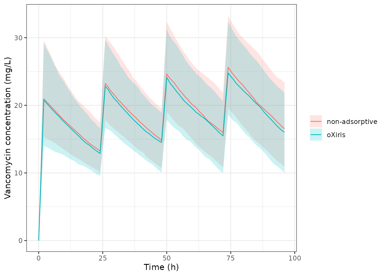
Simulated vancomycin concentrations (median and 5th-95th percentiles) for 2 g loading then 1 g every 24 h, by membrane type, in the virtual Table 1 cohort. The paper’s pcVPC (Figure 2) is on observed TDM data and is not reproduced exactly.
NCA of the virtual cohort
dose_coh <- ev_coh |>
  filter(evid == 1) |>
  left_join(cohort |> select(id, regimen), by = "id")
conc_coh <- PKNCA::PKNCAconc(
  sim_coh |> filter(!is.na(Cc)) |> left_join(cohort |> select(id, regimen), by = "id"),
  Cc ~ time | regimen + FILT_ADSORPTIVE + id
)
nca_coh <- PKNCA::pk.nca(PKNCA::PKNCAdata(
  conc_coh,
  PKNCA::PKNCAdose(dose_coh, amt ~ time | regimen + FILT_ADSORPTIVE + id),
  intervals = data.frame(start = 48, end = 72, auclast = TRUE, cmax = TRUE, cmin = TRUE)
))
nca_tab <- as.data.frame(nca_coh) |>
  filter(PPTESTCD %in% c("auclast", "cmax", "cmin")) |>
  group_by(FILT_ADSORPTIVE, PPTESTCD) |>
  summarise(
    median = median(PPORRES), p05 = quantile(PPORRES, 0.05),
    p95 = quantile(PPORRES, 0.95), .groups = "drop"
  )
nca_tab |>
  mutate(
    membrane = ifelse(FILT_ADSORPTIVE == 1, "oXiris", "non-adsorptive"),
    parameter = dplyr::recode(PPTESTCD,
      auclast = "AUC 48-72 h (mg*h/L)", cmax = "Cmax 48-72 h (mg/L)",
      cmin = "Cmin 48-72 h (mg/L)"
    ),
    across(c(median, p05, p95), \(x) signif(x, 3))
  ) |>
  select(membrane, parameter, median, p05, p95) |>
  dplyr::rename(
    "Membrane" = membrane, "NCA parameter" = parameter,
    "Median" = median, "5th percentile" = p05, "95th percentile" = p95
  ) |>
knitr::kable()| Membrane | NCA parameter | Median | 5th percentile | 95th percentile |
|---|---|---|---|---|
| non-adsorptive | AUC 48-72 h (mg*h/L) | 477.0 | 356.00 | 620.0 |
| non-adsorptive | Cmax 48-72 h (mg/L) | 24.6 | 19.00 | 32.3 |
| non-adsorptive | Cmin 48-72 h (mg/L) | 14.8 | 10.70 | 19.6 |
| oXiris | AUC 48-72 h (mg*h/L) | 463.0 | 341.00 | 601.0 |
| oXiris | Cmax 48-72 h (mg/L) | 24.1 | 17.80 | 31.2 |
| oXiris | Cmin 48-72 h (mg/L) | 14.5 | 9.95 | 18.9 |
The paper reports no NCA table, so the cohort is checked against the model’s own typical value. Over the 48-72 h interval the cohort median AUC sits close to the typical-value AUC of a 60-year-old, because the cohort mean age is 61.5 years and the median of a log-normal clearance is its typical value.
med_auc <- nca_tab |>
  filter(PPTESTCD == "auclast") |>
  left_join(
    auc_typ |> filter(regimen == "2 g LD, 1 g q24h") |> select(FILT_ADSORPTIVE, auc),
    by = "FILT_ADSORPTIVE"
  ) |>
  mutate(pct_diff = 100 * (median / auc - 1))
# Centre, not extremes (vignette guidance). The SE of a median of 200 log-normal
# draws with SD ~0.2 is ~1.8%, and the cohort's age spread adds a few percent of
# Jensen shift; 10% leaves headroom across rxode2 builds and thread counts while
# a mis-transcribed CL or V (tens of percent) still fails.
stopifnot(nrow(med_auc) == 2L, all(abs(med_auc$pct_diff) < 10))
knitr::kable(med_auc |> transmute(
  "oXiris" = FILT_ADSORPTIVE,
  "Cohort median AUC 48-72 h" = round(median, 1),
  "Typical AUC at 60 y" = round(auc, 1),
  "Difference (%)" = round(pct_diff, 1)
))| oXiris | Cohort median AUC 48-72 h | Typical AUC at 60 y | Difference (%) |
|---|---|---|---|
| 0 | 476.6 | 485.3 | -1.8 |
| 1 | 463.1 | 468.9 | -1.2 |
Probability of target attainment (Figure 4)
Figure 4 and Tables S3-S4 were generated with Simulx at a fixed age of 60 years with 10,000 virtual patients per regimen. Here 200 subjects per regimen and membrane arm are simulated at age 60 and AUC(48-72 h)/MIC is compared with 400 mg*h/L.
rxode2::rxSetSeed(20260211)
grid_pta <- tidyr::expand_grid(regimens, FILT_ADSORPTIVE = 0:1, rep = seq_len(n_arm)) |>
  mutate(id = dplyr::row_number(), AGE = 60)
ev_pta <- make_events(grid_pta, seq(48, 72, by = 0.25))
sim_pta <- rxode2::rxSolve(mod, events = ev_pta) |>
  as.data.frame() |>
  select(id, time, Cc) |>
  filter(!is.na(Cc)) |>
  left_join(grid_pta |> select(id, regimen, FILT_ADSORPTIVE), by = "id")
stopifnot(length(unique(sim_pta$id)) == nrow(grid_pta))
auc_pta <- sim_pta |>
  group_by(id, regimen, FILT_ADSORPTIVE) |>
  summarise(auc = sum(diff(time) * (head(Cc, -1) + tail(Cc, -1)) / 2), .groups = "drop")
pta_sim <- tidyr::expand_grid(auc_pta, mic = c(0.25, 0.5, 1, 2, 4)) |>
  group_by(regimen, FILT_ADSORPTIVE, mic) |>
  summarise(pta = 100 * mean(auc / mic > 400), .groups = "drop")
pta_sim |>
  mutate(membrane = ifelse(FILT_ADSORPTIVE == 1, "oXiris", "non-adsorptive")) |>
  ggplot(aes(mic, pta, colour = regimen, linetype = membrane)) +
  geom_line() +
  geom_point(
    data = pta_pub |> filter(target == 400) |>
      mutate(membrane = ifelse(FILT_ADSORPTIVE == 1, "oXiris", "non-adsorptive")),
    aes(y = pta_pub, shape = membrane)
  ) +
  geom_hline(yintercept = 90, linetype = "dashed") +
  scale_x_continuous(trans = "log2", breaks = c(0.25, 0.5, 1, 2, 4)) +
  labs(x = "MIC (mg/L)", y = "PTA (%)", colour = NULL, linetype = NULL, shape = NULL) +
  theme_bw()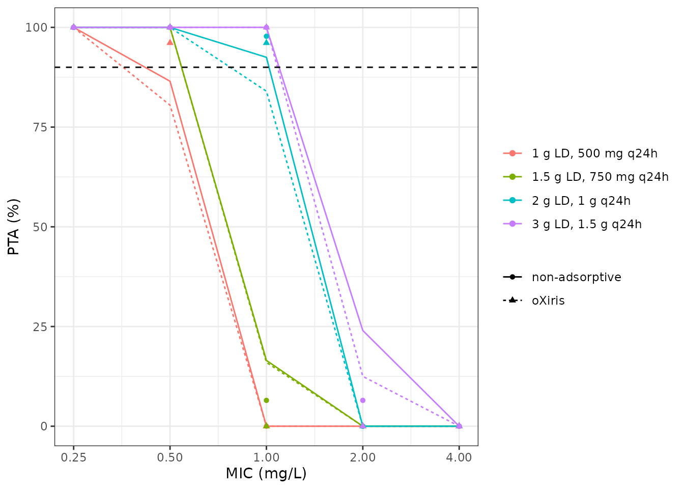
Replicates Figure 4 of Hirunsomboon 2026: PTA for AUC(48-72 h)/MIC > 400 mg*h/L at age 60. Lines: this model (200 subjects per arm). Points: published Table S3 values.
pta_sim |>
  filter(mic %in% c(0.5, 1, 2)) |>
  left_join(pta_pub |> filter(target == 400), by = c("regimen", "FILT_ADSORPTIVE", "mic")) |>
  mutate(
    membrane = ifelse(FILT_ADSORPTIVE == 1, "oXiris", "non-adsorptive"),
    pta = round(pta, 1)
  ) |>
  select(regimen, membrane, mic, pta, pta_pub) |>
  dplyr::rename(
    "Regimen" = regimen, "Membrane" = membrane, "MIC (mg/L)" = mic,
    "PTA, this model (%)" = pta, "PTA, Table S3 (%)" = pta_pub
  ) |>
knitr::kable()| Regimen | Membrane | MIC (mg/L) | PTA, this model (%) | PTA, Table S3 (%) |
|---|---|---|---|---|
| 1 g LD, 500 mg q24h | non-adsorptive | 0.5 | 86.5 | 100.00 |
| 1 g LD, 500 mg q24h | non-adsorptive | 1.0 | 0.0 | 0.00 |
| 1 g LD, 500 mg q24h | non-adsorptive | 2.0 | 0.0 | 0.00 |
| 1 g LD, 500 mg q24h | oXiris | 0.5 | 80.5 | 96.10 |
| 1 g LD, 500 mg q24h | oXiris | 1.0 | 0.0 | 0.00 |
| 1 g LD, 500 mg q24h | oXiris | 2.0 | 0.0 | 0.00 |
| 1.5 g LD, 750 mg q24h | non-adsorptive | 0.5 | 100.0 | 100.00 |
| 1.5 g LD, 750 mg q24h | non-adsorptive | 1.0 | 16.5 | 6.48 |
| 1.5 g LD, 750 mg q24h | non-adsorptive | 2.0 | 0.0 | 0.00 |
| 1.5 g LD, 750 mg q24h | oXiris | 0.5 | 100.0 | 100.00 |
| 1.5 g LD, 750 mg q24h | oXiris | 1.0 | 16.0 | 0.00 |
| 1.5 g LD, 750 mg q24h | oXiris | 2.0 | 0.0 | 0.00 |
| 2 g LD, 1 g q24h | non-adsorptive | 0.5 | 100.0 | 100.00 |
| 2 g LD, 1 g q24h | non-adsorptive | 1.0 | 92.5 | 97.77 |
| 2 g LD, 1 g q24h | non-adsorptive | 2.0 | 0.0 | 0.00 |
| 2 g LD, 1 g q24h | oXiris | 0.5 | 100.0 | 100.00 |
| 2 g LD, 1 g q24h | oXiris | 1.0 | 84.0 | 96.10 |
| 2 g LD, 1 g q24h | oXiris | 2.0 | 0.0 | 0.00 |
| 3 g LD, 1.5 g q24h | non-adsorptive | 0.5 | 100.0 | 100.00 |
| 3 g LD, 1.5 g q24h | non-adsorptive | 1.0 | 100.0 | 100.00 |
| 3 g LD, 1.5 g q24h | non-adsorptive | 2.0 | 24.0 | 6.48 |
| 3 g LD, 1.5 g q24h | oXiris | 0.5 | 100.0 | 100.00 |
| 3 g LD, 1.5 g q24h | oXiris | 1.0 | 100.0 | 100.00 |
| 3 g LD, 1.5 g q24h | oXiris | 2.0 | 12.5 | 0.00 |
pta_cell <- function(reg, mm, mic_val) {
  v <- pta_sim$pta[pta_sim$regimen == reg & pta_sim$FILT_ADSORPTIVE == mm & pta_sim$mic == mic_val]
  if (length(v) != 1L) stop("no unique PTA row for '", reg, "' at MIC ", mic_val)
  v
}
# Spread of log AUC(48-72 h) in this model at a fixed age of 60 years.
sd_log_auc <- auc_pta |>
  group_by(regimen, FILT_ADSORPTIVE) |>
  summarise(s = sd(log(auc)), .groups = "drop") |>
  pull(s) |>
  median()
# The spread of log AUC implied by each published cell that is neither 0 nor
# 100%: PTA = Phi(log(typical AUC / (target * MIC)) / sd), solved for sd. The
# one inconsistent Table S4 cell is left out.
implied_sd <- bracket |>
  filter(pta_pub > 0, pta_pub < 100, uncentered_ok) |>
  mutate(sd = log(auc / (target * mic)) / stats::qnorm(pta_pub / 100)) |>
  pull(sd)
# Deterministic given the published table; robust to the simulated cohort.
stopifnot(
  # Deterministic: 0.062 to 0.096 from the published table and typical AUCs.
  length(implied_sd) == 9L, all(implied_sd > 0.055), all(implied_sd < 0.10),
  sd_log_auc > 0.13, sd_log_auc < 0.22
)
For the typical 60-year-old, the model and the paper agree that every regimen is above the target at MIC 0.5 mg/L and below it at MIC 2 mg/L, and both give the 3 g / 1.5 g regimen 100% attainment at MIC 1 mg/L. Near the threshold the model’s PTA curves are less steep than the published ones. For the recommended 2 g / 1 g regimen at MIC 1 mg/L this simulation gives 92% (non-adsorptive) and 84% (oXiris), close to the 90% line, against the published 97.8% and 96.1%. For 1 g / 500 mg at MIC 0.5 mg/L it gives 86% and 80% against 100% and 96.1%.
In this model, log AUC(48-72 h) has an SD of about 0.15 between subjects of the same age, somewhat below the Table 3 omega for CL (0.20). Back-solving the nine consistent published cells that are neither 0% nor 100% gives SDs between 0.062 and 0.096, and no single value fits them all. The published simulation therefore carried less spread than the Table 3 variances imply. This was not resolved from the paper, so PTA is reported here but not asserted cell by cell. The deterministic bracket check above is the gate.
Assumptions and deviations
-
Uncentered age. The model implements the displayed
equation
CL = 2.82 * exp(-0.007 * Age + 0.053 * MM).lcl = log(2.82)is therefore the intercept atAGE = 0, not the clearance of a typical patient, although the Abstract and Discussion describe 2.82 L/h as the population clearance. The bracket check against Tables S3-S4 above confirms the uncentered reading (79 of 80 cells, against 71 for a centered one). At the cohort mean age of 61.5 years the typical clearance is 1.84 L/h. Age range was not reported; do not extrapolate below adulthood. - IIV scale. Table 3 labels the IIV rows as percentages (21.63, 20.01) but the bootstrap column beside them reports 0.19 and 0.17, and the residual row is printed on the raw scale in both columns. The IIV values are taken as the Monolix omega (SD of eta) multiplied by 100, so the variances are 0.2163^2 and 0.2001^2. Reading them instead as a coefficient of variation would give variances about 2% smaller; nothing downstream depends on the choice.
- Table S3 column order. The two PTA columns of Table S3 are unlabelled; they are read as “with oXiris” then “without”, the order Table S4 labels.
- Published PTA spread and one inconsistent cell. See the PTA section. The supplement’s PTA transitions are steeper than the model’s variances imply, and they are not internally proportional: the 1 g / 500 mg and 2 g / 1 g regimens scale exactly (same 2:1 loading-to-maintenance ratio), so 1 g / 500 mg at MIC 0.5 and 2 g / 1 g at MIC 1 must give the same PTA, yet Table S3 prints 100% and 97.77% for the non-adsorptive arm. The Table S4 cell for 1 g / 500 mg at MIC 0.5 without oXiris (97.8%) is inconsistent with the model under any reading of age. These are properties of the published simulation, not of the model parameters, which are taken verbatim from Table 3.
-
Membrane covariate. The paper’s
MM(oXiris use) is encoded as the canonical binaryFILT_ADSORPTIVE(1 = adsorptive membrane). It applies to patients on CRRT only; the model has no off-CRRT clearance and should not be used for patients off the circuit. - Infusion duration. The fitting dataset’s infusion durations are not reported; the simulations here use the 2 h infusions of Methods 2.4.
-
Screened covariates. Body weight, serum albumin,
residual urine volume and CRRT effluent flow were tested and not
retained (Table S2, Figure S3); they are recorded in
covariatesDataExcluded. - Virtual cohort. Ages are drawn from a normal distribution with the Table 1 mean and SD, restricted to 18-95 years; individual ages are not published.