Midazolam and 1'-OH-midazolam with CYP3A inhibition and induction (Wiebe 2020)
Source:vignettes/articles/Wiebe_2020_midazolam.Rmd
Wiebe_2020_midazolam.Rmd
ui <- rxode2::rxode(readModelDb("Wiebe_2020_midazolam"))
#> ℹ parameter labels from comments will be replaced by 'label()'
#> Warning: some etas defaulted to non-mu referenced, possible parsing error: etaiov_cl_1, etaiov_cl_2, etaiov_cl_3, etaiov_cl_4, etaiov_cl_5, etaiov_cl_1ohm_1, etaiov_cl_1ohm_2, etaiov_cl_1ohm_3, etaiov_cl_1ohm_4, etaiov_cl_1ohm_5, etaiov_fdepot_1, etaiov_fdepot_2, etaiov_fdepot_3, etaiov_fdepot_4, etaiov_fdepot_5
#> as a work-around try putting the mu-referenced expression on a simple line
ui_typ <- rxode2::zeroRe(ui)
#> Warning: some etas defaulted to non-mu referenced, possible parsing error: etaiov_cl_1, etaiov_cl_2, etaiov_cl_3, etaiov_cl_4, etaiov_cl_5, etaiov_cl_1ohm_1, etaiov_cl_1ohm_2, etaiov_cl_1ohm_3, etaiov_cl_1ohm_4, etaiov_cl_1ohm_5, etaiov_fdepot_1, etaiov_fdepot_2, etaiov_fdepot_3, etaiov_fdepot_4, etaiov_fdepot_5
#> as a work-around try putting the mu-referenced expression on a simple line
Model and source
- Citation: Wiebe ST, Meid AD, Mikus G. Composite midazolam and 1’-OH midazolam population pharmacokinetic model for constitutive, inhibited and induced CYP3A activity. J Pharmacokinet Pharmacodyn. 2020;47(6):527-542. doi:10.1007/s10928-020-09704-1. Parameter values from Online Resource 2 (final NONMEM control stream ‘Adopted Composite Model Control Stream with Interaction’).
- Article: https://doi.org/10.1007/s10928-020-09704-1
- Description: Composite parent-metabolite population PK model for midazolam and 1’-OH-midazolam in healthy adults, with CYP3A drug-drug-interaction effects for reversible inhibition (ketoconazole, voriconazole), irreversible inhibition (ritonavir) and induction (efavirenz) (Wiebe 2020). Both analytes have three-compartment disposition. Oral midazolam is absorbed first-order from a depot that simultaneously feeds 1’-OH-midazolam through a pre-systemic formation rate constant; all systemic midazolam clearance forms 1’-OH-midazolam (fraction metabolised fixed to 1). Body weight is a power covariate on the first metabolite intercompartmental clearance. Treatment effects are additive shifts on the typical midazolam central volume, midazolam clearance, bioavailability, pre-systemic formation rate and metabolite clearance. Inter-occasion variability on midazolam clearance, metabolite clearance and bioavailability. Amounts are nmol and concentrations nM. Parameter values are from the deposited final NONMEM control stream (Online Resource 2).
Wiebe 2020 built a joint midazolam / 1’-OH-midazolam model from ten German phase 1 studies in healthy volunteers. The model is meant to detect CYP3A drug-drug interactions from a single midazolam profile. It was built in two stages:
- A composite model for constitutive CYP3A activity:
three-compartment disposition for each analyte, first-order absorption,
a pre-systemic formation rate constant
kmetthat feeds 1’-OH-midazolam directly from the gut / liver, and a fraction metabolised fixed to 1. - An interaction model: every composite parameter was
fixed, and treatment was added as an additive shift on midazolam central
volume, midazolam clearance (
Qmet), bioavailability,kmetand metabolite clearance (CLmet). Inhibition is split into reversible (ketoconazole, voriconazole) and irreversible (ritonavir) effects.
With every treatment indicator at 0, the interaction model reduces exactly to the composite model, so a single model file carries both. The deposited final control stream (Online Resource 2) supplies every value.
Population
pop <- ui$population
tibble::tibble(
  Field = names(pop),
  Value = vapply(pop, function(x) paste(x, collapse = "; "), character(1))
) |>
knitr::kable(caption = "Population metadata (Wiebe 2020 Table 2 and Methods).")| Field | Value |
|---|---|
| species | human |
| n_subjects | 99 |
| n_studies | 7 |
| age_range | 19-52 years |
| age_mean | 26.9 years |
| weight_range | 47-111 kg |
| weight_mean | 71.7 kg |
| sex_female_pct | 40.4 |
| disease_state | healthy volunteers |
| dose_range | Midazolam 3 microgram to 4 mg oral, 1 microgram to 2 mg iv, and semi-simultaneous 4 mg oral followed by 2 mg iv 6 h later; alone or with ketoconazole, voriconazole, ritonavir or efavirenz. |
| regions | Germany (University Hospital Heidelberg) |
| notes | Model development set: 99 healthy adults from seven studies (K119, K155, K169, K257, K380, K194, K345; Table 2), 59 male and 40 female. 2371 midazolam and 2197 1’-OH-midazolam concentrations for constitutive CYP3A activity, plus 1077 and 961 from the inhibition and induction arms (6606 in total). BLQ records were omitted (29 midazolam, 190 1’-OH-midazolam). External validation used 46 more subjects from three limited-sampling studies (K292, K342, K363) and further arms of K119, K169 and K194. NONMEM 7.3, ADVAN6, FOCE-I. The interaction effects were estimated with every composite-model parameter fixed, so the composite model is the special case with all treatment indicators 0. |
The development set contains 99 healthy adults from seven studies (Table 2): mean age 26.9 years (19-52), mean weight 71.7 kg (47-111), 59 men and 40 women. The inhibition arms used ketoconazole 400 mg once daily (K345), voriconazole (K257, K380) and ritonavir 300 mg twice daily (K257, and K119 together with St. John’s wort). The induction arm used efavirenz 400 mg once daily for 14 days (K155, 12 subjects).
Source trace
| Model element | Value | Source |
|---|---|---|
| Structure: 3-cmt parent, 3-cmt metabolite, depot | – | Fig. 1; Online Resource 2 $MODEL,
$DES
|
ka |
2.30635 1/h | Online Resource 2 THETA(6); Table 3 2.31 |
F (bioavailability) |
0.275824 | THETA(7); Table 3 0.276 |
Vc, Vp1, Vp2
|
19.4507, 41.0258, 23.8228 L | THETA(1-3); Table 3 |
Qp1, Qp2
|
8.00001, 46.0527 L/h | THETA(4-5); Table 3 |
Qmet (midazolam CL) |
24.1486 L/h | THETA(10); Table 3 24.1 |
kmet (pre-systemic formation) |
5.31099 1/h | THETA(8); Table 3 5.31 |
Vmet, VMP, VMP2
|
175.643, 684.933, 67.145 L | THETA(9, 12, 14); Table 3 |
QMP (70 kg), QMP2
|
59.5749, 127.374 L/h | THETA(13, 15); Table 3 |
CLmet |
196.827 L/h | THETA(11); Table 3 196.8 |
FM |
1 (fixed) |
$PK FM = 1; Methods |
WT exponent on QMP
|
0.9863 | THETA(24); Table 3 0.986; Methods (70 kg reference) |
Reversible inhibition on Qmet, F,
CLmet
|
-16.336, 0.378806, -64.1022 | THETA(26, 29, 34); Table 3 |
Ritonavir on Vc, Qmet, F,
kmet, CLmet
|
51.8404, -12.67, 1.34248, -5.23662, 1117.36 | THETA(25, 27, 30, 32, 35); Table 3 |
Induction on Qmet, F,
kmet
|
37.9834, -0.200032, 12.4264 | THETA(28, 31, 33); Table 3 |
IIV block Vmet, Vc
|
0.158449, 0.109819, 0.142583 |
$OMEGA BLOCK(2); Table 3 prints SDs and
correlation |
IIV Qmet, CLmet, Vp1,
Qp1, F, kmet,
QMP
|
0.0087203, 0.0176367, 0.167708, 0.251747, 0.0545658, 0.135776, 0.235254 |
$OMEGA; Table 3 prints SDs |
IOV Qmet, CLmet, F (5
occasions) |
0.0231946, 0.0859661, 0.0261532 |
$OMEGA BLOCK(1) + SAME; Table 3 prints
SDs |
| Proportional SDs, early / late, no inhibition | MDZ 0.503162 / 0.148938; 1’-OH 0.555696 / 0.215375 | THETA(16, 20, 18, 22); Table 3 |
| Proportional SDs, early / late, inhibition | 0.482949 / 0.267324 | THETA(36, 38); Table 3 |
| 1’-OH additive SD | 0.00001 nM | THETA(19, 23) |
| Early/late split | 0.5 h (1.5 h with inhibition) |
$ERROR; Results |
Virtual cohort and helpers
MW_MIDAZOLAM <- 325.77                        # g/mol
mg_to_nmol <- function(mg) mg * 1e-3 / MW_MIDAZOLAM * 1e9

CONDITIONS <- tibble::tribble(
  ~condition,               ~CONMED_KETOCONAZOLE, ~CONMED_VORICONAZOLE, ~CONMED_RTV, ~CONMED_CYP3A4_IND,
  "Baseline",               0,                    0,                    0,           0,
  "Reversible (keto/vori)", 1,                    0,                    0,           0,
  "Irreversible (ritonavir)", 0,                  0,                    1,           0,
  "Induction (efavirenz)",  0,                    0,                    0,           1
)

#' One subject's event table. `doses` is a data frame of time / amt / cmt;
#' observations sit on the `central` ODE state with dvid 1, and rxode2
#' returns both Cc and Cc_1ohm on every observation row.
make_events <- function(doses, times, condition = "Baseline", id = 1L, WT = 70) {
  dose <- data.frame(id = id, time = doses$time, amt = doses$amt,
                     cmt = doses$cmt, evid = 1L, dvid = NA_integer_)
  obs <- data.frame(id = id, time = times, amt = NA_real_, cmt = "central",
                    evid = 0L, dvid = 1L)
  ev <- rbind(dose, obs)
  cov <- CONDITIONS[CONDITIONS$condition == condition, ]
  for (nm in setdiff(names(cov), "condition")) ev[[nm]] <- cov[[nm]]
  ev$WT <- WT
  ev$OCC <- 1L
  ev$condition <- condition
  ev[order(ev$time, -ev$evid), ]
}

oral_4mg <- data.frame(time = 0, amt = mg_to_nmol(4), cmt = "depot")
iv_2mg <- data.frame(time = 0, amt = mg_to_nmol(2), cmt = "central")
oral_iv <- data.frame(time = c(0, 6), amt = mg_to_nmol(c(4, 2)),
                      cmt = c("depot", "central"))

solve_typical <- function(events, model = ui_typ) {
  suppressMessages(as.data.frame(rxode2::rxSolve(
    model, events, useLinCmt = FALSE, keep = "condition",
    returnType = "data.frame"
  )))
}
All typical-value solves use a 70 kg subject (the weight reference) on occasion 1.
Replicate Figure 3
Figure 3 of Wiebe 2020 shows visual predictive checks for the final interaction model, with data normalised to a 4 mg midazolam dose. The typical-value curves below reproduce its panels: base oral, base iv, base oral + iv, inhibition, and induction.
TIMES <- sort(unique(c(seq(0, 2, by = 0.05), seq(2, 25, by = 0.25))))

fig3 <- bind_rows(
  solve_typical(make_events(oral_4mg, TIMES)) |> mutate(panel = "Base - oral"),
  solve_typical(make_events(iv_2mg, TIMES)) |>
    mutate(Cc = 2 * Cc, Cc_1ohm = 2 * Cc_1ohm, panel = "Base - iv (x2)"),
  solve_typical(make_events(oral_iv, TIMES)) |> mutate(panel = "Base - oral + iv"),
  solve_typical(make_events(oral_4mg, TIMES, "Reversible (keto/vori)")) |>
    mutate(panel = "Reversible inhibition - oral"),
  solve_typical(make_events(oral_4mg, TIMES, "Irreversible (ritonavir)")) |>
    mutate(panel = "Irreversible inhibition - oral"),
  solve_typical(make_events(oral_4mg, TIMES, "Induction (efavirenz)")) |>
    mutate(panel = "Induction - oral")
)

fig3 |>
  filter(time > 0) |>
  select(time, panel, Midazolam = Cc, `1'-OH-midazolam` = Cc_1ohm) |>
  pivot_longer(c(Midazolam, `1'-OH-midazolam`), names_to = "analyte",
               values_to = "conc") |>
  ggplot(aes(time, conc, colour = analyte)) +
  geom_line() +
  scale_y_log10() +
  facet_wrap(~panel, ncol = 2) +
  labs(x = "Time (h)", y = "Concentration (nM)", colour = NULL,
       caption = "Replicates the typical course of Figure 3 of Wiebe 2020 (4 mg-normalised).") +
  theme_bw() +
  theme(legend.position = "bottom")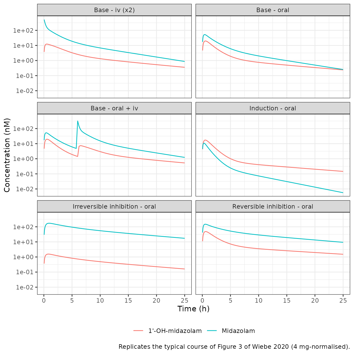
The pre-systemic formation route: which reading of the control stream
The deposited control stream does not write the depot the way Figure
1 draws it. In $PK it sets KA = THETA(6) on
midazolam records and KA = KMET on metabolite records, and
in $DES:
DADT(1) = -KA*A(1)
DADT(2) =  KA*A(1) - ...
DADT(5) =  KMET*A(1) + K2M*A(2) - ...
NONMEM integrates each interval with the $PK values of
the record that closes it. Which KA applies therefore
depends on the record order in the (unpublished) dataset. There are two
readings:
-
Reading A (encoded). The intervals close on
midazolam records. The depot empties at
ka= 2.31 1/h into midazolam, and 1’-OH-midazolam gainskmet * depotin parallel without draining the depot. -
Reading B. The intervals close on metabolite
records. The depot then empties at
kmetinto both midazolam and 1’-OH-midazolam, andTHETA(6)would never enter the likelihood.
Table 3 reports ka with an RSE of 4.44%, which is
impossible if THETA(6) never enters the fit, so the control stream
itself rules out Reading B. Figure 3 gives a second, independent check.
The maintainers digitised the observed median of the “Base - Oral Dose”
panels (midazolam and 1’-OH-midazolam, 4 mg-normalised) from the
published figure image. Reading B is built from the same model by
re-routing the depot:
reading_b <- function(events) {
  d <- solve_typical(events)
  # Reading B: depot drains at kmet into BOTH analytes. Solve it with a
  # stand-alone ODE on the same typical parameters.
  m <- rxode2::rxode2({
    d/dt(depot) <- -kmet_p * depot
    d/dt(central) <- kmet_p * depot - (q + q2 + cl) / vc * central +
      q / vp * p1 + q2 / vp2 * p2
    d/dt(p1) <- q / vc * central - q / vp * p1
    d/dt(p2) <- q2 / vc * central - q2 / vp2 * p2
    d/dt(met) <- kmet_p * depot + cl / vc * central -
      (cl_1ohm + q_1ohm + q2_1ohm) / vc_1ohm * met +
      q_1ohm / vp_1ohm * mp1 + q2_1ohm / vp2_1ohm * mp2
    d/dt(mp1) <- q_1ohm / vc_1ohm * met - q_1ohm / vp_1ohm * mp1
    d/dt(mp2) <- q2_1ohm / vc_1ohm * met - q2_1ohm / vp2_1ohm * mp2
    f(depot) <- fdepot
    Cc <- central / vc
    Cc_1ohm <- met / vc_1ohm
  })
  pars <- c(kmet_p = 5.31099, q = 8.00001, q2 = 46.0527, cl = 24.1486,
            vc = 19.4507, vp = 41.0258, vp2 = 23.8228, cl_1ohm = 196.827,
            q_1ohm = 59.5749, q2_1ohm = 127.374, vc_1ohm = 175.643,
            vp_1ohm = 684.933, vp2_1ohm = 67.145, fdepot = 0.275824)
  ev <- rxode2::et(amt = mg_to_nmol(4), cmt = "depot") |>
    rxode2::et(unique(d$time[d$time > 0]))
  as.data.frame(rxode2::rxSolve(m, ev, params = pars))
}

# Digitised by the maintainers from the Wiebe 2020 Figure 3 image, panels
# 'Midazolam Base - Oral Dose' and "1'-OH Midazolam Base - Oral Dose", solid
# line = observed median. Approximate (log axis, low-resolution image).
fig3_digitised <- tibble::tribble(
  ~time, ~mdz_obs, ~oh_obs,
  0.75,  40,       18,
  5,     5,        1.5,
  10,    1.6,      0.75,
  24,    0.22,     0.18
)

sim_a <- solve_typical(make_events(oral_4mg, fig3_digitised$time))
sim_b <- reading_b(make_events(oral_4mg, fig3_digitised$time))

cmp <- fig3_digitised |>
  mutate(
    mdz_A = sim_a$Cc[match(time, sim_a$time)],
    oh_A = sim_a$Cc_1ohm[match(time, sim_a$time)],
    mdz_B = sim_b$Cc[match(time, sim_b$time)],
    oh_B = sim_b$Cc_1ohm[match(time, sim_b$time)]
  )

cmp |>
  mutate(across(-time, ~ signif(.x, 3))) |>
  rename(
    "Time (h)" = time,
    "MDZ, Fig. 3 (nM)" = mdz_obs, "MDZ, reading A" = mdz_A, "MDZ, reading B" = mdz_B,
    "1'-OH, Fig. 3 (nM)" = oh_obs, "1'-OH, reading A" = oh_A, "1'-OH, reading B" = oh_B
  ) |>
knitr::kable(caption = "Typical-value predictions of both readings against the digitised Figure 3 medians (4 mg oral).")| Time (h) | MDZ, Fig. 3 (nM) | 1’-OH, Fig. 3 (nM) | MDZ, reading A | 1’-OH, reading A | MDZ, reading B | 1’-OH, reading B |
|---|---|---|---|---|---|---|
| 0.75 | 40.00 | 18.00 | 46.000 | 19.000 | 44.000 | 10.300 |
| 5.00 | 5.00 | 1.50 | 6.110 | 1.930 | 5.560 | 1.300 |
| 10.00 | 1.60 | 0.75 | 2.020 | 0.758 | 1.940 | 0.533 |
| 24.00 | 0.22 | 0.18 | 0.291 | 0.257 | 0.281 | 0.171 |
sse <- function(pred, obs) sum(log(pred / obs)^2)
score <- c(
  A = sse(cmp$oh_A, cmp$oh_obs),
  B = sse(cmp$oh_B, cmp$oh_obs)
)
score
#>         A         B
#> 0.1919386 0.4510089
stopifnot(
  # Reading A fits the 1'-OH-midazolam medians better than reading B
  score[["A"]] < score[["B"]],
  # and its peak-region value is within 25% of the digitised median.
  abs(cmp$oh_A[cmp$time == 0.75] / cmp$oh_obs[cmp$time == 0.75] - 1) < 0.25,
  # Midazolam itself is nearly identical under both readings (the
  # disagreement is confined to the metabolite): typical value within a
  # factor of 1.6 of the digitised median at every time.
  all(abs(log(cmp$mdz_A / cmp$mdz_obs)) < log(1.6))
)
The two readings give almost the same midazolam profile. They differ
in how much 1’-OH-midazolam is formed pre-systemically. Under reading A,
an oral dose forms F * Dose * (1 + kmet/ka) = 0.91 x Dose
of metabolite. Under reading B it forms only F * Dose =
0.28 x Dose. Reading A reproduces the Figure 3 metabolite peak of about
18 nM at 0.75 h (19 nM), while reading B under-predicts it by 43%.
Midazolam clearance cut-points (Table 4)
Wiebe 2020 proposes classifying CYP3A modulation from the
model-estimated midazolam clearance Qmet: 4.82-16.4 L/h
inhibition, 16.4-41.8 L/h no modulation, 41.8-88.9 L/h induction
(Abstract; Table 4). The typical Qmet of each treatment
category must fall in its own bin.
typ_cl <- bind_rows(lapply(CONDITIONS$condition, function(cn) {
  d <- solve_typical(make_events(oral_4mg, 1, cn))
  data.frame(condition = cn, cl = d$cl[1], fdepot = d$fdepot[1],
             vc = d$vc[1], k_1ohm_form = d$k_1ohm_form[1], cl_1ohm = d$cl_1ohm[1])
}))
typ_cl$bin <- cut(typ_cl$cl, c(4.82, 16.4, 41.8, 88.9),
                  labels = c("Inhibition", "No modulation", "Induction"))

typ_cl |>
  mutate(across(where(is.numeric), ~ signif(.x, 4))) |>
  rename("Condition" = condition, "Qmet (L/h)" = cl, "F" = fdepot,
         "Vc (L)" = vc, "kmet (1/h)" = k_1ohm_form, "CLmet (L/h)" = cl_1ohm,
         "Table 4 bin" = bin) |>
knitr::kable(caption = "Typical parameter values per treatment category.")| Condition | Qmet (L/h) | F | Vc (L) | kmet (1/h) | CLmet (L/h) | Table 4 bin |
|---|---|---|---|---|---|---|
| Baseline | 24.150 | 0.27580 | 19.45 | 5.31100 | 196.8 | No modulation |
| Reversible (keto/vori) | 7.813 | 0.65460 | 19.45 | 5.31100 | 132.7 | Inhibition |
| Irreversible (ritonavir) | 11.480 | 1.61800 | 71.29 | 0.07437 | 1314.0 | Inhibition |
| Induction (efavirenz) | 62.130 | 0.07579 | 19.45 | 17.74000 | 196.8 | Induction |
stopifnot(
  identical(as.character(typ_cl$bin),
            c("No modulation", "Inhibition", "Inhibition", "Induction")),
  # Results text: 'Estimated bioavailability of midazolam was 27.6% and
  # clearance was 24.1 L/h'.
  abs(typ_cl$fdepot[1] - 0.276) < 0.001,
  abs(typ_cl$cl[1] - 24.1) < 0.05
)
Irreversible inhibition drives the typical bioavailability to 1.62. That is above 1 and not physically meaningful. It is what the published additive coefficient gives, and it is kept as published (see Assumptions and deviations).
PKNCA validation
The paper reports no NCA table, so the NCA is scored against the model’s own exposure identities, which are exact for this linear system:
- midazolam:
AUC(0-inf) = F * Dose / Qmet; - 1’-OH-midazolam after oral dosing:
AUC(0-inf) = F * Dose * (1 + kmet / ka) / CLmet, i.e. the systemically formed part (FM = 1) plus the pre-systemic partkmet * integral(depot); - 1’-OH-midazolam after iv dosing:
AUC(0-inf) = Dose / CLmet.
NCA_GRID <- sort(unique(c(seq(0, 4, by = 0.02), seq(4, 48, by = 0.25),
                          seq(48, 240, by = 2))))
arms <- tibble::tribble(
  ~treatment,          ~condition,                 ~route,
  "Baseline oral",     "Baseline",                 "oral",
  "Baseline iv",       "Baseline",                 "iv",
  "Reversible oral",   "Reversible (keto/vori)",   "oral",
  "Ritonavir oral",    "Irreversible (ritonavir)", "oral",
  "Induction oral",    "Induction (efavirenz)",    "oral"
)

nca_sim <- bind_rows(lapply(seq_len(nrow(arms)), function(i) {
  doses <- if (arms$route[i] == "oral") oral_4mg else iv_2mg
  solve_typical(make_events(doses, NCA_GRID, arms$condition[i])) |>
    mutate(treatment = arms$treatment[i], id = 1L,
           dose_nmol = doses$amt[1])
}))

run_nca <- function(conc_col) {
  conc <- nca_sim |>
    filter(!is.na(.data[[conc_col]])) |>
    transmute(id, treatment, time, conc = .data[[conc_col]])
  conc <- bind_rows(conc, conc |> distinct(id, treatment) |> mutate(time = 0, conc = 0)) |>
    distinct(id, treatment, time, .keep_all = TRUE) |>
    arrange(treatment, id, time)
  dose_df <- nca_sim |> distinct(id, treatment, dose_nmol) |>
    mutate(time = 0)
  conc_obj <- PKNCA::PKNCAconc(conc, conc ~ time | treatment + id,
                               concu = "nM", timeu = "h")
  dose_obj <- PKNCA::PKNCAdose(dose_df, dose_nmol ~ time | treatment + id,
                               doseu = "nmol")
  intervals <- data.frame(start = 0, end = Inf, cmax = TRUE, tmax = TRUE,
                          aucinf.obs = TRUE, half.life = TRUE)
  res <- PKNCA::pk.nca(PKNCA::PKNCAdata(conc_obj, dose_obj, intervals = intervals))
  as.data.frame(res$result) |>
    select(treatment, PPTESTCD, PPORRES) |>
    pivot_wider(names_from = PPTESTCD, values_from = PPORRES)
}

nca_parent <- run_nca("Cc")
nca_metab <- run_nca("Cc_1ohm")

ka <- 2.30635
expected <- nca_sim |>
  group_by(treatment) |>
  slice(1) |>
  ungroup() |>
  left_join(arms, by = "treatment") |>
  transmute(
    treatment,
    parent_auc = ifelse(route == "oral", fdepot, 1) * dose_nmol / cl,
    metab_auc = ifelse(route == "oral",
                       fdepot * dose_nmol * (1 + k_1ohm_form / ka),
                       dose_nmol) / cl_1ohm
  )

nca_tbl <- expected |>
  left_join(nca_parent |> select(treatment, parent_nca = aucinf.obs,
                                 parent_cmax = cmax, parent_tmax = tmax,
                                 parent_thalf = half.life), by = "treatment") |>
  left_join(nca_metab |> select(treatment, metab_nca = aucinf.obs,
                                metab_cmax = cmax), by = "treatment")

nca_tbl |>
  mutate(across(where(is.numeric), ~ signif(.x, 4))) |>
  rename(
    "Arm (4 mg oral / 2 mg iv)" = treatment,
    "MDZ AUCinf, identity (nM*h)" = parent_auc,
    "MDZ AUCinf, NCA (nM*h)" = parent_nca,
    "MDZ Cmax (nM)" = parent_cmax,
    "MDZ Tmax (h)" = parent_tmax,
    "MDZ t1/2 (h)" = parent_thalf,
    "1'-OH AUCinf, identity (nM*h)" = metab_auc,
    "1'-OH AUCinf, NCA (nM*h)" = metab_nca,
    "1'-OH Cmax (nM)" = metab_cmax
  ) |>
knitr::kable(caption = "PKNCA results against the closed-form exposure identities (typical values, 70 kg).")| Arm (4 mg oral / 2 mg iv) | MDZ AUCinf, identity (nM*h) | 1’-OH AUCinf, identity (nM*h) | MDZ AUCinf, NCA (nM*h) | MDZ Cmax (nM) | MDZ Tmax (h) | MDZ t1/2 (h) | 1’-OH AUCinf, NCA (nM*h) | 1’-OH Cmax (nM) |
|---|---|---|---|---|---|---|---|---|
| Baseline iv | 254.20 | 31.19 | 254.30 | 315.60 | 0.00 | 5.116 | 31.19 | 6.156 |
| Baseline oral | 140.20 | 56.83 | 140.20 | 52.41 | 0.42 | 5.117 | 56.83 | 19.740 |
| Induction oral | 14.98 | 41.09 | 14.97 | 10.78 | 0.30 | 4.069 | 41.09 | 17.330 |
| Reversible oral | 1029.00 | 200.00 | 1029.00 | 148.40 | 0.52 | 9.647 | 200.00 | 48.510 |
| Ritonavir oral | 1731.00 | 15.61 | 1731.00 | 172.20 | 0.92 | 9.672 | 15.61 | 1.557 |
# The two sides use the same parameters; the difference is pure numerical
# (trapezoidal / extrapolation) error, so a tight bound is correct.
stopifnot(
  all(abs(nca_tbl$parent_nca / nca_tbl$parent_auc - 1) < 0.01),
  all(abs(nca_tbl$metab_nca / nca_tbl$metab_auc - 1) < 0.01)
)
auc_ratio <- function(arm) {
  nca_tbl$parent_nca[nca_tbl$treatment == arm] /
    nca_tbl$parent_nca[nca_tbl$treatment == "Baseline oral"]
}
auc_ratios <- c(
  reversible = auc_ratio("Reversible oral"),
  ritonavir = auc_ratio("Ritonavir oral"),
  induction = auc_ratio("Induction oral")
)
round(auc_ratios, 3)
#> reversible  ritonavir  induction
#>      7.336     12.344      0.107
Relative to baseline, reversible inhibition raises typical oral midazolam AUC 7.3-fold and ritonavir 12.3-fold, while induction lowers it 9.4-fold. These sizes correspond to the potent modulators of the development data.
Stochastic simulation
A stochastic check with between-subject, inter-occasion and residual variability, 100 subjects per arm, on the Figure 3 “Base - Oral Dose” and “Inhibition - Oral Dose” designs (4 mg oral).
set.seed(97041)
rxode2::rxSetSeed(97041)
N_PER_ARM <- 100
VPC_TIMES <- c(0.25, 0.5, 0.75, 1, 1.5, 2, 2.5, 3, 4, 6, 8, 10, 24)

vpc_events <- bind_rows(
  lapply(seq_len(N_PER_ARM), function(i)
    make_events(oral_4mg, VPC_TIMES, "Baseline", id = i,
                WT = stats::runif(1, 47, 111))),
  lapply(seq_len(N_PER_ARM), function(i)
    make_events(oral_4mg, VPC_TIMES, "Irreversible (ritonavir)", id = N_PER_ARM + i,
                WT = stats::runif(1, 47, 111)))
)

vpc <- as.data.frame(rxode2::rxSolve(ui, vpc_events, useLinCmt = FALSE,
                                     keep = "condition", returnType = "data.frame"))

vpc_sum <- vpc |>
  filter(time > 0) |>
  select(id, time, condition, Midazolam = Cc, `1'-OH-midazolam` = Cc_1ohm) |>
  pivot_longer(c(Midazolam, `1'-OH-midazolam`), names_to = "analyte",
               values_to = "conc") |>
  group_by(condition, analyte, time) |>
  summarise(q05 = quantile(conc, 0.05), q50 = median(conc),
            q95 = quantile(conc, 0.95), .groups = "drop")

ggplot(vpc_sum, aes(time, q50)) +
  geom_ribbon(aes(ymin = q05, ymax = q95), alpha = 0.25) +
  geom_line() +
  scale_y_log10() +
  facet_grid(analyte ~ condition) +
  labs(x = "Time (h)", y = "Concentration (nM)",
       caption = "Simulated median and 90% interval (individual predictions), 4 mg oral midazolam.") +
  theme_bw()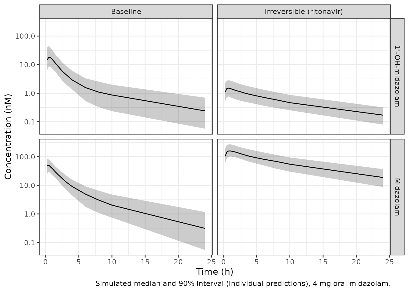
Assumptions and deviations
-
Parameter source. All values come from the
deposited final control stream (Online Resource 2). They agree with
Table 3 once Table 3’s variability rows are read correctly. Its
“omega^2” column prints standard deviations (sqrt of the
$OMEGAvariances), and its “omega^2 Vmet * omega^2 Vc” row prints the correlation (0.731), not the covariance (0.1098). The printed 95% CI of that row (0.264-0.392) matches neither and was not used. -
Pre-systemic formation route. The model encodes the
as-run control stream (reading A above): 1’-OH-midazolam gains
kmet * depotwithout draining the depot. It is not the mass-conserving branching of Figure 1. The choice rests on the estimableka(Table 3 RSE 4.44%) and on the Figure 3 metabolite peak. -
Treatment covariates. The control stream carries
one three-way treatment code (
TRT3), so its categories never overlap. The model maps them to concomitant-medication indicators: reversible inhibition =CONMED_KETOCONAZOLEorCONMED_VORICONAZOLE; irreversible inhibition =CONMED_RTV(in study K119 this was ritonavir plus St. John’s wort, net inhibition); induction =CONMED_CYP3A4_IND, estimated from 14-day efavirenz. Do not set more than one category on the same record. The paper applied the induction effect to other inducers only in external validation, where it over-predicted the induction effect for weak inducers. - Non-physical bioavailability under ritonavir. The additive ritonavir shift on F (+1.342) gives a typical F of 1.62. It is kept as published. With IIV and IOV on F, individual values above 1 also occur under reversible inhibition.
-
Residual error. The control stream uses
W = sqrt(FPROP^2 * IPRED^2 + FADD^2)with$SIGMA 1 FIX, so each FPROP is a standard deviation whose sign does not matter. The two negative estimates (-0.215375, -0.267324) are stored as magnitudes. The early/late split uses the control stream’sTIME, taken here as time since the occasion’s first midazolam dose (tin the model). Simulate each occasion from its own time origin. The inhibition error terms apply to both kinds of inhibition (control streamTRT = 2). The 1e-5 nM additive term for 1’-OH-midazolam is applied on all records. In the control stream it is 0 on inhibition records, a negligible difference. -
Occasions. The five IOV slots per parameter follow
the control stream’s
$ABBREVIATED REPLACEmapping. Simulations here useOCC = 1. - Concentration units. The control stream does not state units. Amounts in nmol and concentrations in nM are inferred from Figure 3 (nM axis, 4 mg normalisation). With molar amounts, the fixed fraction metabolised of 1 is a molar balance. The typical-value curves reproduce the Figure 3 magnitudes.
-
Covariates not retained. An age effect on
kmetwas found but not retained (no reduction in variability), and sex was not significant (Results). Neither is in the model.