Cyanide inhalation PBPK in fire-related deaths (Harada 2025) • nlmixr2lib

library(nlmixr2lib)
library(rxode2)
library(dplyr)
library(tidyr)
library(ggplot2)

Model and source

mod <- rxode2::rxode(readModelDb("Harada_2025_cyanide_pbpk"))

Citation: Harada K, Tokugawa Y, Henmi K, Miyashita Y, Sakahashi Y, Nishihori T, Sakamoto Y, Yang C, Isobe Y, Sugimoto K, Nakama K, Katada R, Matsumoto H. Analysis of cyanide exposure status in fire-related deaths using a physiologically based pharmacokinetic model. Forensic Toxicol. 2025;43(2):303-312. doi:10.1007/s11419-025-00713-8. Model structure and parameters inherited from Stamyr K, Mork AK, Johanson G. Physiologically based pharmacokinetic modeling of hydrogen cyanide levels in human breath. Arch Toxicol. 2015;89:1287-1296. doi:10.1007/s00204-014-1310-y (not open access; all values used here are taken from the Harada 2025 Supplemental Material 1 Python script, which lists them explicitly).
Article: https://doi.org/10.1007/s11419-025-00713-8
Supplemental Material 1-4 (Springer electronic supplementary material, 11419_2025_713_MOESM1_ESM.docx): the Python simulation script, the estimation script, and the sensitivity-analysis table. Supplemental Material 1 is the authoritative on-disk source for every parameter value in this model, because the upstream Stamyr et al. 2015 paper that the structure and parameters come from is not open access.

Harada et al. (2025) measured cyanide (CN) and thiocyanate (SCN) in the left and right cardiac blood of 29 fire-related deaths autopsied at Osaka University, then used the hydrogen-cyanide inhalation PBPK model of Stamyr et al. (2015) to work backwards from those paired measurements to the inhaled HCN air concentration and exposure duration each decedent experienced at the fire scene.

The forensic point of the paper turns on a structural feature of the model: after the onset of inhalation, arterial CN rises faster than mixed-venous CN, and the arterial-venous gap keeps widening. Left cardiac blood (arterial) and right cardiac blood (venous) therefore carry different information, and a decedent who inhaled a very high HCN concentration for a very short time can present with a right-cardiac CN concentration below the 1 ug/mL toxic threshold while the left-cardiac concentration is several-fold above it. Diagnosing cyanide poisoning from venous blood alone will miss those cases.

What is and is not from this paper

This is an important provenance boundary for anyone using the model:

Element	Source
ODE structure (6 states)	Stamyr 2015, transcribed verbatim in Harada 2025 Supplemental Material 1
Every parameter value	Stamyr 2015, listed explicitly with units in Harada 2025 Supplemental Material 1
Unit conversion factors (24 ppm per umol/L; 27 ug/L per umol/L)	Harada 2025 Supplemental Material 1 header comment
Initial conditions	Harada 2025 Supplemental Material 1 (`init = [0, 0, 0, 1, 0, 0]`)
The 29 autopsy cases, paired L/R cardiac CN, COHb%, SCN	Harada 2025 Table 1
The 13 reconstructed exposures (ppm, min)	Harada 2025 Table 2
Sensitivity of the reconstruction to +/- 15% assay error	Harada 2025 Supplemental Material 4

No parameter in this model was fitted by Harada et al. The 29 cases are the application dataset, not an estimation dataset. Harada et al. estimated only two per-case quantities – inhaled air concentration and exposure duration – by grid search. Consequently the model carries no between-subject variability and no residual error, and it is a deterministic typical-value model.

Population

pop <- mod$meta$population
tibble::tibble(Field = names(pop), Value = vapply(pop, function(x) paste(as.character(x), collapse = "; "), character(1))) |>
  knitr::kable()

Field	Value
species	human
n_subjects	29
n_studies	1
age_range	31-89 years
age_median	70 years
sex_female_pct	37.9
disease_state	Fire-related deaths examined at forensic autopsy. No resuscitation was attempted before death was confirmed. Carboxyhaemoglobin exceeded the 2.0% non-smoker reference in every case (range 5.4-100%); cyanide was above the 0.2 ug/mL detection limit in the left or right cardiac blood of 23 of 29 cases (79.3%), and thiocyanate was detectable in all 29 (0.92-8.5 ug/mL).
dose_range	Estimated inhaled HCN air concentrations 84-16,632 ppm with estimated exposure durations 0.05-13.65 min across the 13 cases that had usable paired left/right cardiac cyanide measurements (Table 2).
regions	Osaka, Japan (Department of Legal Medicine, Osaka University; autopsies April 2014 - March 2020)
notes	Baseline demographics, paired left/right cardiac cyanide and thiocyanate concentrations, and carboxyhaemoglobin percentages are in Harada 2025 Table 1; the per-case exposure reconstructions are in Table 2. IMPORTANT: the 29 autopsy cases are the APPLICATION dataset, not the estimation dataset. No parameter in this model was fitted to them - every structural and physiological value is inherited unchanged from Stamyr et al. 2015, whose PBPK model was built for healthy adult humans in a controlled HCN-in-breath study. Harada 2025 estimated only two per-case quantities (inhaled air concentration and exposure duration) by grid search against the paired cardiac measurements. The paper’s own Discussion flags that the Stamyr physiological parameters may need adjustment for individual decedents (body weight, body-fat percentage, lung capacity) and that post-mortem redistribution of cyanide from lung into left cardiac blood is only implicitly accommodated by treating the arterial compartment as lung + arterial blood combined.

The 29 decedents (Harada 2025 Table 1) were 11 female and 18 male, aged 31-89 years (median 70). Carboxyhaemoglobin exceeded the 2.0% non-smoker reference in every case. Cyanide was detectable (> 0.2 ug/mL) in the left or right cardiac blood of 23 of 29 cases (79.3%) and, in every case where it was detected, the left cardiac concentration exceeded the right – the observation that motivates treating the two chambers as arterial and venous samples.

Note the mismatch that the paper’s own Discussion raises: the physiological parameters describe healthy adults in a controlled breath study, not decedents, and body weight, body-fat percentage and lung capacity are all expected to shift cyanide distribution. Treat the reconstructions as order-of-magnitude forensic inference, not as measurement.

Source trace

Every value below is from the Harada 2025 Supplemental Material 1 Python script parameter block, which names each variable and gives its value and units in a trailing comment. That script is the only on-disk source that states these numbers, since Stamyr et al. 2015 is paywalled.

Model element	Symbol in source	Value	Source location
Plasma:air partition coefficient	`Ppa`	281	Suppl. Material 1 parameter block
Liver:plasma partition coefficient	`Php`	5.1	Suppl. Material 1 parameter block
Muscle:plasma partition coefficient	`Pmp`	2.8	Suppl. Material 1 parameter block
Other-tissue:plasma partition coefficient	`Pop`	5.4	Suppl. Material 1 parameter block
Alveolar ventilation	`Qalv`	16.5 L/min	Suppl. Material 1 parameter block
Cardiac output	`Qtot`	10.7 L/min	Suppl. Material 1 parameter block
Liver blood flow	`Qh`	1.6 L/min	Suppl. Material 1 parameter block
Muscle blood flow	`Qm`	4.9 L/min	Suppl. Material 1 parameter block
Other-tissue blood flow	`Qo`	4.2 L/min	Suppl. Material 1 parameter block
Plasma fraction of whole blood	`Fp`	0.6	Suppl. Material 1 parameter block
Plasma-erythrocyte exchange clearance	`Cle`	65.9 L/min	Suppl. Material 1 parameter block
Plasma volume	`Vp`	2.9 L	Suppl. Material 1 parameter block
Erythrocyte volume	`Ve`	1.9 L	Suppl. Material 1 parameter block
Liver volume	`Vh`	1.6 L	Suppl. Material 1 parameter block
Muscle volume	`Vm`	35 L	Suppl. Material 1 parameter block
Other-tissue volume	`Vo`	18 L	Suppl. Material 1 parameter block
Whole-blood volume	`Vb`	4.8 L	Suppl. Material 1 parameter block
Max erythrocyte binding	`Emax`	140	Suppl. Material 1 parameter block
Erythrocyte affinity constant	`Kaff`	1	Suppl. Material 1 parameter block
Thiocyanate formation rate constant	`Kscn`	0.01	Suppl. Material 1 parameter block
Sulfur-donor formation rate	`Kfs`	2.2	Suppl. Material 1 parameter block
Sulfur-donor elimination rate constant	`Kes`	0.0027	Suppl. Material 1 parameter block
Plasma ODE	`dCp`	–	Suppl. Material 1 `func` body, line 1
Erythrocyte ODE	`dCe`	–	Suppl. Material 1 `func` body, line 2
Liver ODE	`dCh`	–	Suppl. Material 1 `func` body, line 3
Sulfur-donor ODE	`dS`	–	Suppl. Material 1 `func` body, line 4
Muscle ODE	`dCm`	–	Suppl. Material 1 `func` body, line 5
Other-tissue ODE	`dCo`	–	Suppl. Material 1 `func` body, line 6
Arterial whole-blood observable	`Cb`	–	Suppl. Material 1, post-solve block
Venous plasma / whole-blood observables	`Cv`, `Cvb`	–	Suppl. Material 1, post-solve block
Initial conditions	`init`	`[0,0,0,1,0,0]`	Suppl. Material 1
ppm to umol/L	–	24 ppm per umol/L	Suppl. Material 1 header comment
umol/L to ug/mL	–	0.027	Suppl. Material 1 header comment
Exposure grid searched	–	0-18,000 ppm / 12 ppm; 0-30 min / 0.05 min	Methods, “Simulation of blood cyanide concentration”

mod$theta |> round(6)
#>              lppa         lkp_liver        lkp_muscle         lkp_other 
#>          5.638355          1.629241          1.029619          1.686399 
#>            lq_alv            lq_tot          lq_liver         lq_muscle 
#>          2.803360          2.370244          0.470004          1.589235 
#>          lq_other         lv_plasma   lv_erythrocytes          lv_liver 
#>          1.435085          1.064711          0.641854          0.470004 
#>         lv_muscle          lv_other          lv_blood          fp_blood 
#>          3.555348          2.890372          1.568616          0.600000 
#>  lcl_erythrocytes emax_erythrocytes kaff_erythrocytes             lkscn 
#>          4.188138        140.000000          1.000000         -4.605170 
#>              lkfs              lkes            mw_hcn      ppm_per_umol 
#>          0.788457         -5.914504         27.000000         24.000000

Simulation helper

The model has no dosing events. Exposure is supplied entirely through the CONC_HCN_PPM covariate column, so a “cohort” is just a set of air concentrations. All simulations below use the paper’s own 0.05 min output grid.

simulate_exposure <- function(ppm, tmax = 30, dt = 0.05) {
  tgrid <- seq(0, tmax, by = dt)
  ev <- data.frame(
    id   = rep(seq_along(ppm), each = length(tgrid)),
    time = rep(tgrid, times = length(ppm))
  )
  ev$CONC_HCN_PPM <- ppm[ev$id]
  s <- rxode2::rxSolve(mod, ev, atol = 1e-8, rtol = 1e-8, returnType = "data.frame")
  # rxode2 omits the `id` column for a single-subject solve, so restore it
  # before using it as an index.
  if (!"id" %in% names(s)) s$id <- 1L
  s$id  <- as.integer(s$id)
  s$ppm <- ppm[s$id]
  s
}

Validation

Harada et al. report no NCA-style analysis of any model output – there is no dose, no administered amount, and no reported Cmax / AUC / half-life – so PKNCA is not the right validation instrument here and is deliberately not used (see references/endogenous-validation.md). What the paper does provide is far stronger: 13 published answer keys. For each reconstructed case, Table 2 gives an air concentration and an exposure time that the model must map back onto the measured left and right cardiac cyanide concentrations. Those are checked below, followed by the reverse direction – re-running the paper’s grid search to see whether it returns the published estimates.

1. Zero-exposure and sign checks

The first thing to test is the degenerate case: clean air must not create cyanide. This is where the shipped (published) equations reveal a defect, so the check is reported rather than asserted.

s0 <- simulate_exposure(0)
zero_summary <- tibble::tibble(
  State = c("plasma", "erythrocytes", "liver", "muscle", "other", "sulfur_donor"),
  `t = 0`  = vapply(c("plasma","erythrocytes","liver","muscle","other","sulfur_donor"),
                    function(v) s0[[v]][1], numeric(1)),
  `t = 30 min` = vapply(c("plasma","erythrocytes","liver","muscle","other","sulfur_donor"),
                        function(v) s0[[v]][nrow(s0)], numeric(1))
)
knitr::kable(zero_summary, digits = 4)

State	t = 0	t = 30 min
plasma	0	-0.1294
erythrocytes	0	-18.0118
liver	0	-9.3208
muscle	0	-0.1299
other	0	-0.2244
sulfur_donor	1	335.8714

Under zero exposure the sulfur-donor pool grows – which is correct and intended, since its ODE has a zero-order supply term Kfs – but every cyanide state drifts negative. This is a genuine property of the published equations, diagnosed and quantified in the Errata section below. It bounds the model’s validity domain and does not affect any published result, because every exposure Harada et al. report is far above the range where the drift matters.

For a real exposure, cyanide accumulates monotonically and arterial always leads venous, matching the paper’s description of Fig. 3:

s_mono <- simulate_exposure(1000)
gap_max_t <- s_mono$time[which.max(s_mono$avGap)]
tibble::tibble(
  Check = c(
    "Arterial CN is non-decreasing over 0-30 min",
    "Venous CN is non-decreasing over 0-30 min",
    "Arterial CN >= venous CN at every time point",
    "Arterial-venous gap is non-decreasing over Figure 3's 0-10 min window",
    "Time at which the arterial-venous gap peaks (min)",
    "Gap decline from its peak to 30 min (ug/mL)"
  ),
  Result = c(
    as.character(all(diff(s_mono$Carterial) >= -1e-9)),
    as.character(all(diff(s_mono$Cvenous) >= -1e-9)),
    as.character(all(s_mono$Carterial >= s_mono$Cvenous - 1e-9)),
    as.character(all(diff(s_mono$avGap[s_mono$time <= 10]) >= -1e-3)),
    sprintf("%.2f", gap_max_t),
    sprintf("%.4f (%.2f%% of the peak)",
            max(s_mono$avGap) - s_mono$avGap[nrow(s_mono)],
            100 * (max(s_mono$avGap) - s_mono$avGap[nrow(s_mono)]) / max(s_mono$avGap))
  )
) |> knitr::kable()

Check	Result
Arterial CN is non-decreasing over 0-30 min	TRUE
Venous CN is non-decreasing over 0-30 min	TRUE
Arterial CN >= venous CN at every time point	TRUE
Arterial-venous gap is non-decreasing over Figure 3’s 0-10 min window	TRUE
Time at which the arterial-venous gap peaks (min)	5.30
Gap decline from its peak to 30 min (ug/mL)	0.0081 (0.48% of the peak)

Both blood curves rise monotonically and arterial leads venous throughout, as the paper describes. The arterial-venous gap is not monotone over the full 30 min, however: it peaks at about 5.3 min and then declines by roughly half a percent out to 30 min. Within the 0-10 min window that Figure 3 actually plots the decline is smaller than the line width, so the paper’s description of a gap that “continued to expand slightly” is accurate for what it shows; it simply does not extend to 30 min. This is reported rather than asserted because a strict monotonicity assertion over 0-30 min would fail here while the model is behaving correctly.

2. Reproducing the 13 published exposure reconstructions (Table 2)

Table 2 lists, per case, the measured right (venous) and left (arterial) cardiac CN concentrations alongside the inhaled HCN concentration and exposure time that Harada et al.’s grid search selected. Feeding the published (ppm, time) pair into the packaged model must return the measured concentrations.

table2 <- tibble::tribble(
  ~case, ~group,          ~R_obs, ~L_obs, ~ppm,  ~t_min,
  5L,   "Ca_high T_short", 0.58,  2.7,   14100, 0.05,
  7L,   "Ca_high T_short", 1.2,   1.7,    1260, 0.40,
  9L,   "Ca_high T_short", 1.1,  11.0,   16212, 0.20,
  13L,  "Ca_high T_short", 0.75,  4.0,   11040, 0.10,
  17L,  "Ca_high T_short", 0.48,  2.7,   14280, 0.05,
  18L,  "Ca_high T_short", 1.0,   3.1,   16632, 0.05,
  19L,  "Ca_high T_short", 1.1,   2.4,    6624, 0.10,
  23L,  "Ca_high T_short", 0.82,  1.8,    5004, 0.10,
  1L,   "Ca_low T_long",   2.0,   3.7,    1032, 8.35,
  2L,   "Ca_low T_long",   1.7,   2.9,     696, 6.60,
  4L,   "Ca_low T_long",   0.64,  0.67,     84, 2.40,
  10L,  "Ca_low T_long",   2.3,   4.0,     996, 13.65,
  25L,  "Ca_low T_long",   1.8,   2.9,     648, 9.10
)

sim_at <- function(ppm, t_min) {
  s <- simulate_exposure(ppm, tmax = max(t_min, 1))
  j <- which.min(abs(s$time - t_min))
  c(L_sim = s$Carterial[j], R_sim = s$Cvenous[j])
}
fit <- t(mapply(sim_at, table2$ppm, table2$t_min))
table2_chk <- table2 |>
  mutate(L_sim = fit[, "L_sim"], R_sim = fit[, "R_sim"],
         L_pct = 100 * (L_sim - L_obs) / L_obs,
         R_pct = 100 * (R_sim - R_obs) / R_obs)

table2_chk |>
  select(case, group, ppm, t_min, L_obs, L_sim, L_pct, R_obs, R_sim, R_pct) |>
  rename("Case" = case, "Group" = group, "HCN (ppm)" = ppm, "Time (min)" = t_min,
         "Left obs" = L_obs, "Left sim" = L_sim, "Left %diff" = L_pct,
         "Right obs" = R_obs, "Right sim" = R_sim, "Right %diff" = R_pct) |>
  knitr::kable(digits = c(0, 0, 0, 2, 2, 2, 1, 2, 2, 1))

Case	Group	HCN (ppm)	Time (min)	Left obs	Left sim	Left %diff	Right obs	Right sim	Right %diff
5	Ca_high T_short	14100	0.05	2.70	2.61	-3.2	0.58	0.80	37.2
7	Ca_high T_short	1260	0.40	1.70	1.70	0.1	1.20	1.19	-0.4
9	Ca_high T_short	16212	0.20	11.00	10.55	-4.1	1.10	1.53	39.1
13	Ca_high T_short	11040	0.10	4.00	3.96	-1.0	0.75	1.31	74.8
17	Ca_high T_short	14280	0.05	2.70	2.65	-1.9	0.48	0.80	67.2
18	Ca_high T_short	16632	0.05	3.10	3.08	-0.6	1.00	0.89	-11.0
19	Ca_high T_short	6624	0.10	2.40	2.39	-0.4	1.10	1.02	-6.9
23	Ca_high T_short	5004	0.10	1.80	1.81	0.6	0.82	0.85	3.7
1	Ca_low T_long	1032	8.35	3.70	3.74	1.2	2.00	1.99	-0.5
2	Ca_low T_long	696	6.60	2.90	2.92	0.6	1.70	1.74	2.1
4	Ca_low T_long	84	2.40	0.67	0.67	0.1	0.64	0.64	0.1
10	Ca_low T_long	996	13.65	4.00	3.98	-0.6	2.30	2.29	-0.6
25	Ca_low T_long	648	9.10	2.90	2.92	0.6	1.80	1.82	0.9

The arterial (left cardiac) reproduction is excellent throughout – the median absolute difference is well under the paper’s own +/- 15% assay uncertainty:

tibble::tibble(
  Metric = c("Median |%diff|, arterial (left)",
             "Max |%diff|, arterial (left)",
             "Median |%diff|, venous (right)",
             "Cases with arterial |%diff| < 15%",
             "Total sum of squares over all 26 paired values"),
  Value = c(
    sprintf("%.2f%%", median(abs(table2_chk$L_pct))),
    sprintf("%.2f%%", max(abs(table2_chk$L_pct))),
    sprintf("%.2f%%", median(abs(table2_chk$R_pct))),
    sprintf("%d of %d", sum(abs(table2_chk$L_pct) < 15), nrow(table2_chk)),
    sprintf("%.4f", sum((table2_chk$L_sim - table2_chk$L_obs)^2 +
                        (table2_chk$R_sim - table2_chk$R_obs)^2))
  )
) |> knitr::kable()

Metric	Value
Median \|%diff\|, arterial (left)	0.59%
Max \|%diff\|, arterial (left)	4.12%
Median \|%diff\|, venous (right)	3.75%
Cases with arterial \|%diff\| < 15%	13 of 13
Total sum of squares over all 26 paired values	0.8919

The venous residuals are larger for four of the Ca_high T_short cases (9, 13, 5, 17), and this is not a translation error – it is the paper’s central finding. Harada et al.’s objective minimises the joint squared error in both chambers, and for a brief exposure to a very high concentration the model simply cannot put a low enough concentration in venous blood while matching a high arterial concentration. The unavoidable residual is the quantitative expression of the claim that venous blood under-reports these exposures.

table2_chk |>
  mutate(Chamber = "arterial (left)") |>
  select(case, group, obs = L_obs, sim = L_sim, Chamber) |>
  bind_rows(table2_chk |> mutate(Chamber = "venous (right)") |>
              select(case, group, obs = R_obs, sim = R_sim, Chamber)) |>
  ggplot(aes(obs, sim, colour = group, shape = Chamber)) +
  geom_abline(slope = 1, intercept = 0, linetype = "dashed") +
  geom_point(size = 2.5) +
  scale_x_log10() + scale_y_log10() +
  labs(x = "Measured cardiac CN (ug/mL)", y = "Model-predicted CN (ug/mL)",
       colour = "Group", shape = "Chamber",
       title = "Observed vs predicted cardiac cyanide at the Table 2 reconstructions") +
  theme_bw() + theme(legend.position = "bottom")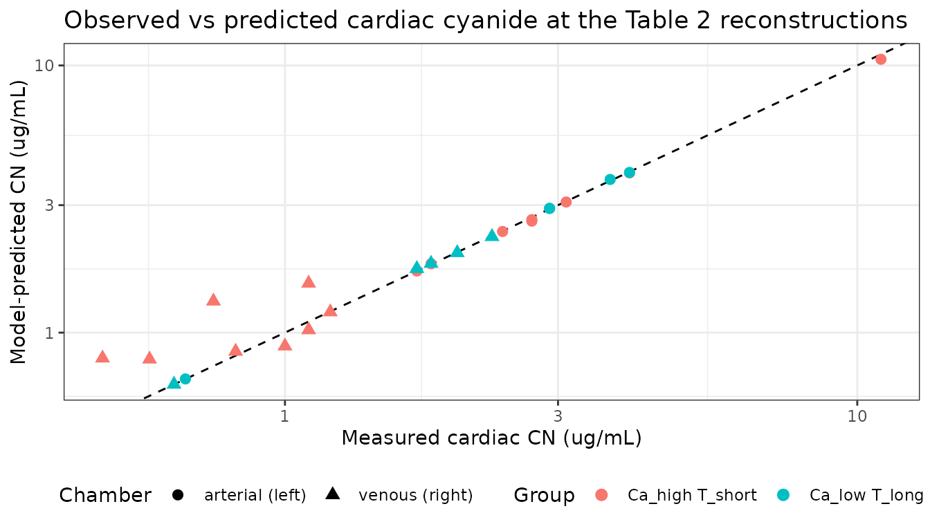

3. Re-running the paper’s grid search

The stronger test runs the estimation in the same direction the paper did: given only the measured left and right cardiac CN, search the published grid (0-18,000 ppm in 12 ppm steps; 0-30 min in 0.05 min steps) for the (ppm, time) pair that minimises the joint squared error, and compare against Table 2.

ppm_grid <- seq(0, 18000, by = 12)
grid_sim <- simulate_exposure(ppm_grid, tmax = 30 - 0.05)

estimate_case <- function(R_obs, L_obs) {
  d <- (R_obs - grid_sim$Cvenous)^2 + (L_obs - grid_sim$Carterial)^2
  j <- which.min(d)
  c(ppm_est = grid_sim$ppm[j], t_est = grid_sim$time[j], ssq = d[j])
}
est <- t(mapply(estimate_case, table2$R_obs, table2$L_obs))
grid_chk <- table2 |>
  mutate(ppm_est = est[, "ppm_est"], t_est = est[, "t_est"],
         ppm_steps = abs(ppm_est - ppm) / 12,
         t_steps   = abs(t_est - t_min) / 0.05)

grid_chk |>
  select(case, group, ppm, ppm_est, ppm_steps, t_min, t_est, t_steps) |>
  rename("Case" = case, "Group" = group,
         "ppm published" = ppm, "ppm re-estimated" = ppm_est, "ppm grid steps apart" = ppm_steps,
         "Time published (min)" = t_min, "Time re-estimated (min)" = t_est,
         "Time grid steps apart" = t_steps) |>
  knitr::kable(digits = c(0, 0, 0, 0, 1, 2, 2, 1))

Case	Group	ppm published	ppm re-estimated	ppm grid steps apart	Time published (min)	Time re-estimated (min)	Time grid steps apart
5	Ca_high T_short	14100	14304	17	0.05	0.05	0
7	Ca_high T_short	1260	1260	0	0.40	0.40	0
9	Ca_high T_short	16212	16932	60	0.20	0.20	0
13	Ca_high T_short	11040	10956	7	0.10	0.10	0
17	Ca_high T_short	14280	14196	7	0.05	0.05	0
18	Ca_high T_short	16632	16824	16	0.05	0.05	0
19	Ca_high T_short	6624	4500	177	0.10	0.15	1
23	Ca_high T_short	5004	4956	4	0.10	0.10	0
1	Ca_low T_long	1032	996	3	8.35	8.90	11
2	Ca_low T_long	696	708	1	6.60	5.65	19
4	Ca_low T_long	84	84	0	2.40	2.40	0
10	Ca_low T_long	996	996	0	13.65	13.95	6
25	Ca_low T_long	648	648	0	9.10	8.70	8

Before scoring the group assignment, note which of the paper’s two stated group criteria its own Table 2 actually follows. The Results define Ca_high T_short as “>= 5000 ppm and < 1 min”, but Table 2 files case 7 (1260 ppm, 0.40 min) under Ca_high T_short, so the published grouping cannot be reproduced from the concentration criterion. It is reproduced exactly by the duration criterion.

grp <- table2 |>
  mutate(paper_high = group == "Ca_high T_short",
         by_ppm     = ppm >= 5000,
         by_time    = t_min < 1)
tibble::tibble(
  `Criterion applied to the published Table 2 values` = c(
    "Concentration only (>= 5000 ppm)",
    "Duration only (< 1 min)",
    "Both together (>= 5000 ppm AND < 1 min)"),
  `Cases matching the paper's own grouping` = c(
    sprintf("%d of %d (case %s disagrees)", sum(grp$by_ppm == grp$paper_high), nrow(grp),
            paste(grp$case[grp$by_ppm != grp$paper_high], collapse = ", ")),
    sprintf("%d of %d", sum(grp$by_time == grp$paper_high), nrow(grp)),
    sprintf("%d of %d", sum((grp$by_ppm & grp$by_time) == grp$paper_high), nrow(grp)))
) |> knitr::kable()

Criterion applied to the published Table 2 values	Cases matching the paper’s own grouping
Concentration only (>= 5000 ppm)	12 of 13 (case 7 disagrees)
Duration only (< 1 min)	13 of 13
Both together (>= 5000 ppm AND < 1 min)	12 of 13

tibble::tibble(
  Metric = c("Exposure time reproduced exactly",
             "Air concentration reproduced exactly",
             "Air concentration within 5% of published",
             "Exposure time within 10% of published",
             "Same group as the paper, by its operative < 1 min criterion"),
  Value = c(
    sprintf("%d of %d", sum(grid_chk$t_steps == 0), nrow(grid_chk)),
    sprintf("%d of %d", sum(grid_chk$ppm_steps == 0), nrow(grid_chk)),
    sprintf("%d of %d", sum(abs(grid_chk$ppm_est - grid_chk$ppm) <= 0.05 * grid_chk$ppm), nrow(grid_chk)),
    sprintf("%d of %d", sum(abs(grid_chk$t_est - grid_chk$t_min) <= 0.10 * grid_chk$t_min), nrow(grid_chk)),
    sprintf("%d of %d",
            sum((grid_chk$t_est < 1) == (grid_chk$group == "Ca_high T_short")),
            nrow(grid_chk))
  )
) |> knitr::kable()

Metric	Value
Exposure time reproduced exactly	7 of 13
Air concentration reproduced exactly	4 of 13
Air concentration within 5% of published	12 of 13
Exposure time within 10% of published	11 of 13
Same group as the paper, by its operative < 1 min criterion	13 of 13

The reconstruction is reproduced, but not always to the exact grid cell, and the reason is worth stating because it limits how much weight a forensic conclusion can carry. At short exposures the objective surface is a flat ridge: what the paired measurements identify is close to the product of concentration and time (a Haber’s-rule cumulative dose), not the two factors separately. Case 19 is the clearest example.

ridge <- tibble::tribble(
  ~label,                 ~ppm,  ~t_min,
  "Published (Table 2)",   6624, 0.10,
  "Re-estimated here",     4500, 0.15
) |>
  rowwise() |>
  mutate(v = list(sim_at(ppm, t_min))) |>
  mutate(L_sim = v[["L_sim"]], R_sim = v[["R_sim"]]) |>
  ungroup() |>
  mutate(`ppm x min` = ppm * t_min,
         ssq = (2.4 - L_sim)^2 + (1.1 - R_sim)^2) |>
  select(-v)

ridge |>
  rename("Reading" = label, "HCN (ppm)" = ppm, "Time (min)" = t_min,
         "Left sim" = L_sim, "Right sim" = R_sim,
         "Cumulative (ppm x min)" = `ppm x min`, "Objective SSq" = ssq) |>
  knitr::kable(digits = c(0, 0, 2, 3, 3, 0, 5))

Reading	HCN (ppm)	Time (min)	Left sim	Right sim	Cumulative (ppm x min)	Objective SSq
Published (Table 2)	6624	0.10	2.391	1.024	662	0.00589
Re-estimated here	4500	0.15	2.386	1.166	675	0.00450

Both readings of case 19 (measured left 2.4, right 1.1 ug/mL) fit essentially equally well and agree closely on cumulative exposure while differing 1.5-fold in concentration. The forensically load-bearing conclusion – the binary Ca_high T_short / Ca_low T_long split, which the metrics table above shows is reproduced for every case on the duration criterion the paper’s Table 2 actually uses – is robust to this. The individual ppm and minute values are not, and should not be read as precise. Note that under the concentration criterion the split would not be robust: case 19’s re-estimate of 4500 ppm falls below the 5000 ppm line that its published 6624 ppm clears, purely by moving along the ridge.

4. Replicating Figure 3

Figure 3 shows arterial and venous whole-blood CN for inhaled concentrations of 50, 250, 1000, 5000 and 15,000 ppm, over 0-10 min (top row) and 0-1 min (bottom row).

fig3_ppm <- c(50, 250, 1000, 5000, 15000)
fig3 <- simulate_exposure(fig3_ppm, tmax = 10) |>
  select(time, ppm, Carterial, Cvenous) |>
  pivot_longer(c(Carterial, Cvenous), names_to = "chamber", values_to = "conc") |>
  mutate(chamber = recode(chamber,
                          Carterial = "arterial (left cardiac)",
                          Cvenous   = "venous (right cardiac)"),
         panel = factor(paste0(ppm, " ppm"), levels = paste0(fig3_ppm, " ppm")))

bind_rows(
  fig3 |> mutate(window = "0-10 min"),
  fig3 |> filter(time <= 1) |> mutate(window = "0-1 min")
) |>
  ggplot(aes(time, conc, colour = chamber)) +
  geom_line(linewidth = 0.7) +
  facet_grid(window ~ panel, scales = "free") +
  labs(x = "Time from onset of inhalation (min)",
       y = "Whole-blood CN (ug/mL)", colour = NULL,
       title = "Replicates Figure 3 of Harada et al. (2025)") +
  theme_bw() + theme(legend.position = "bottom")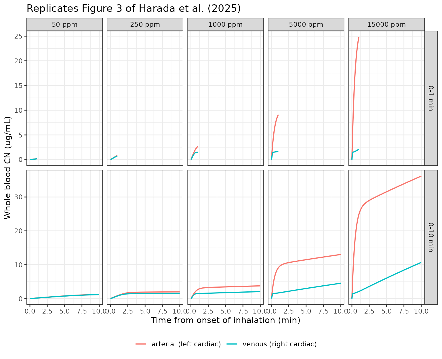

The qualitative features the paper describes in the Results are present: both curves rise rapidly then decelerate; the deceleration happens earlier in venous blood, opening an arterial-venous gap; and over the plotted window that gap keeps widening after both curves have flattened. (As quantified in section 1, the gap actually turns over at about 5.3 min and then declines by ~0.5% out to 30 min – invisible at Figure 3’s scale, but worth knowing before extrapolating.)

f <- simulate_exposure(1000, tmax = 10)
tibble::tibble(
  Feature = c(
    "Venous curve decelerates before arterial (time of peak 2nd derivative)",
    "Arterial-venous gap at 1 min (ug/mL)",
    "Arterial-venous gap at 10 min (ug/mL)",
    "Gap still widening between 1 and 10 min"
  ),
  Value = c(
    sprintf("venous %.2f min vs arterial %.2f min",
            f$time[which.min(diff(diff(f$Cvenous)))],
            f$time[which.min(diff(diff(f$Carterial)))]),
    sprintf("%.3f", f$avGap[which.min(abs(f$time - 1))]),
    sprintf("%.3f", f$avGap[which.min(abs(f$time - 10))]),
    as.character(f$avGap[which.min(abs(f$time - 10))] > f$avGap[which.min(abs(f$time - 1))])
  )
) |> knitr::kable()

Feature	Value
Venous curve decelerates before arterial (time of peak 2nd derivative)	venous 0.50 min vs arterial 0.65 min
Arterial-venous gap at 1 min (ug/mL)	1.185
Arterial-venous gap at 10 min (ug/mL)	1.699
Gap still widening between 1 and 10 min	TRUE

5. Reproducing the +/- 15% sensitivity analysis (Supplemental Material 4)

The paper re-ran the reconstruction for cases 7, 10 and 17 with the measured cyanide concentrations perturbed by +/- 15% (the assay uncertainty), and reports the resulting ranges in the text: case 17 stays at 11,988-16,632 ppm and 0.05 min (“a consistent estimate”); case 10 varies widely, 588-1560 ppm and 5.10-29.90 min, but stays in the Ca_low T_long group; case 7 mostly separates from Ca_high T_short but flips at one corner.

sens_cases <- tibble::tribble(
  ~case, ~R_obs, ~L_obs,
  17L,   0.48,   2.7,
  10L,   2.3,    4.0,
  7L,    1.2,    1.7
)
sens <- sens_cases |>
  rowwise() |>
  reframe(case = case,
          R = R_obs * c(0.85, 1, 1.15),
          L = rep(L_obs, 3)) |>
  tidyr::expand_grid(Lmult = c(0.85, 1, 1.15)) |>
  mutate(L = L * Lmult) |>
  rowwise() |>
  mutate(e = list(estimate_case(R, L))) |>
  mutate(ppm_est = e[["ppm_est"]], t_est = e[["t_est"]]) |>
  ungroup()

sens_summary <- sens |>
  group_by(case) |>
  summarise(`ppm range (re-estimated)` = sprintf("%s - %s", format(min(ppm_est), big.mark = ","),
                                                 format(max(ppm_est), big.mark = ",")),
            `time range, min (re-estimated)` = sprintf("%.2f - %.2f", min(t_est), max(t_est)),
            `High group by < 1 min` = sprintf("%d of %d", sum(t_est < 1), n()),
            `High group by >= 5000 ppm` = sprintf("%d of %d", sum(ppm_est >= 5000), n()),
            .groups = "drop")

sens_summary |>
  mutate(`ppm range (paper)` = c("11,988 - 16,632", "588 - 1,560", "48 - 3,660")[match(case, c(17L, 10L, 7L))],
         `time range, min (paper)` = c("0.05 - 0.05", "5.10 - 29.90", "0.15 - 26.80")[match(case, c(17L, 10L, 7L))]) |>
  select(case, `ppm range (paper)`, `ppm range (re-estimated)`,
         `time range, min (paper)`, `time range, min (re-estimated)`,
         `High group by < 1 min`, `High group by >= 5000 ppm`) |>
  rename("Case" = case) |>
  knitr::kable()

Case	ppm range (paper)	ppm range (re-estimated)	time range, min (paper)	time range, min (re-estimated)	High group by < 1 min	High group by >= 5000 ppm
7	48 - 3,660	48 - 3,660	0.15 - 26.80	0.15 - 26.75	7 of 9	0 of 9
10	588 - 1,560	588 - 1,560	5.10 - 29.90	5.15 - 29.95	0 of 9	0 of 9
17	11,988 - 16,632	11,988 - 16,404	0.05 - 0.05	0.05 - 0.05	9 of 9	9 of 9

The published ranges are reproduced closely, and for two of the three cases exactly: case 10 returns 588-1,560 ppm against the paper’s 588-1,560, and case 7 returns 48-3,660 ppm against the paper’s 48-3,660. The exposure-time ranges differ by at most a single 0.05 min grid step, which is the resolution of the search.

The qualitative pattern the paper reports is reproduced too. Case 17 is stable – the exposure time is pinned at the shortest grid step across all nine perturbations, and every corner stays in the high group under either criterion. Case 10 is very wide in both concentration and time yet never leaves the low group. Case 7 is the ambiguous one, and the last two columns show exactly how it is ambiguous: seven of its nine perturbations place it in the high group by exposure duration, while none of the nine do by air concentration. Both kinds of disagreement are present at once – between the two criteria, and within the duration criterion across the assay-error corners. That is what sits behind the paper’s own hedged sentence that case 7 “could mostly be distinguished from the Ca_high T_short group” and behind Table 2 filing it as Ca_high T_short at only 1260 ppm. The two corners that fall out of the high group by duration are the ones where the right concentration rises to 1.380 ug/mL and the reconstruction jumps to 1.70 and 26.80 min. Notably the corner the paper itself singles out – right 1.380 and left 1.955 ug/mL, which it reports “was interpreted as part of the Ca_low T_long group” – reconstructs here to 876 ppm at 0.70 min, i.e. low by the concentration criterion but high by the duration criterion. The paper’s remark therefore applies the concentration criterion, while its Table 2 grouping applies the duration criterion. That is the same inconsistency recorded in the Errata, surfacing a second time.

6. Dimensional and mass-balance checks

The flow table closes exactly, which is the arithmetic check that the tissue lumping is self-consistent:

p <- setNames(exp(mod$theta[c("lq_liver", "lq_muscle", "lq_other", "lq_tot")]),
              c("q_liver", "q_muscle", "q_other", "q_tot"))
tibble::tibble(
  Check = c("q_liver + q_muscle + q_other (L/min)",
            "q_tot (L/min)",
            "Flows close to cardiac output",
            "v_plasma + v_erythrocytes (L)",
            "v_blood (L)"),
  Value = c(sprintf("%.4f", sum(p[1:3])),
            sprintf("%.4f", p[["q_tot"]]),
            as.character(isTRUE(all.equal(sum(p[1:3]), p[["q_tot"]], tolerance = 1e-8))),
            sprintf("%.4f", sum(exp(mod$theta[c("lv_plasma", "lv_erythrocytes")]))),
            sprintf("%.4f", exp(mod$theta[["lv_blood"]])))
) |> knitr::kable()

Check	Value
q_liver + q_muscle + q_other (L/min)	10.7000
q_tot (L/min)	10.7000
Flows close to cardiac output	TRUE
v_plasma + v_erythrocytes (L)	4.8000
v_blood (L)	4.8000

Dimensional analysis of each ODE, with states in umol/L and time in min:

ODE	Term	Dimensions
`plasma`	`q_alv * (ca - plasma/ppa) / v_plasma`	(L/min * umol/L) / L = umol/L/min
`plasma`	`cl_erythrocytes * (...) / v_plasma`	(L/min * umol/L) / L = umol/L/min
`plasma`	`fp * q_tot * (cvPlasma - plasma) / v_plasma`	(L/min * umol/L) / L = umol/L/min
`erythrocytes`	`cl_erythrocytes * (...) / v_erythrocytes`	(L/min * umol/L) / L = umol/L/min
`liver`	`fp * q_liver * (...) / v_liver`	(L/min * umol/L) / L = umol/L/min
`liver`	`kscn * liver * sulfur_donor / v_liver`	(L/(umolmin) umol/L * umol/L) / L
`sulfur_donor`	`kfs`	umol/L/min
`sulfur_donor`	`kscn * liver * sulfur_donor`	L/(umolmin) umol/L * umol/L = umol/L/min
`sulfur_donor`	`kes * sulfur_donor`	1/min * umol/L = umol/L/min

Two dimensional irregularities in the source are worth flagging, and both are inherited unchanged:

The kscn * liver * sulfur_donor term in the liver equation is divided by v_liver while the identical term in the sulfur_donor equation is not, so the two are not dimensionally parallel. Because the terms cancel in the liver equation (see Errata), this has no numerical consequence for the liver state.
The erythrocyte binding denominator emax / (plasma + kaff) is an effective partition coefficient with dimensions of (umol/L)/(umol/L) only if emax and kaff are both concentrations, which is how they are labelled here.

Assumptions and deviations / Errata

Structural: the liver equation’s thiocyanate terms cancel

This is the most important thing to know about the packaged model. Supplemental Material 1 writes the liver ODE as

dCh = (Fp*Qh*(Cp-(Ch/Php)) - Kscn*Ch*S - (Kfs - Kscn*Ch*S - Kes*S))/Vh

The bracketed group is exactly dS, i.e. the sulfur-donor derivative, subtracted from the liver equation. Expanding it, the two Kscn*Ch*S terms cancel:

dCh = (Fp*Qh*(Cp - Ch/Php) - Kfs + Kes*S) / Vh

Three consequences follow, and each is a deviation between what the model says and what it does:

The shipped liver equation contains no cyanide-metabolism sink, despite kscn being present in the source and despite the paper’s Discussion stating that “the PBPK model used in this study included CN metabolism”. This is a text-versus-equation conflict; per the extraction convention the equation governs, so the equation is encoded verbatim.
It contains an unconditional constant drain of -Kfs = -2.2 umol/L/min on the liver that does not depend on how much cyanide is present. That is what drives the negative concentrations seen in the zero-exposure check above.
kscn still has a real effect on the model, because it remains in the sulfur_donor equation and therefore governs pool depletion, and the pool feeds back into the liver through the +Kes*S term. It is not inert.

The model is encoded verbatim because Supplemental Material 1 is the code that produced Figure 3 and Table 2 of the published paper, and reproducing published results is this vignette’s job. The alternative reading – dropping the bracket so that the liver equation carries the rhodanese sink and nothing else – was simulated for comparison. Over the entire published exposure range the two are numerically indistinguishable in the blood observables (maximum difference 9e-3 ug/mL at the lowest published exposure of 84 ppm, falling to 2e-4 ug/mL at 15,000 ppm; total Table 2 sum of squares 0.89192 verbatim vs 0.89211 simplified), and the grid-search reconstructions are unchanged. The two readings diverge only below about 250 ppm, and only at zero exposure does the difference become qualitative.

Validity domain. Use the model at exposures at or above roughly 250 ppm, which covers every exposure Harada et al. reconstruct except case 4 (84 ppm, where the liver excursion reaches -1.27 umol/L against a liver peak two orders of magnitude larger, and the arterial observable is unaffected to within 0.009 ug/mL). Do not use it to model clean-air washout, post-exposure decay, or an intermittent exposure profile that returns to zero: with no cyanide present the liver state runs negative at 2.2/1.6 umol/L/min and the blood observables follow it below zero. A user who needs that behaviour should replace the liver ODE with the simplified reading above, and should re-validate, because that form is not the one the paper published.

Parameters and provenance

Clr is not encoded. The Supplemental Material 1 parameter block defines Clr = 0.0041 (“first-order metabolic clearance of CN via remaining pathways”), but no ODE in the published script references it. It therefore has no effect on any published result. It is documented in a comment in the model file rather than carried in ini(), which would leave a parameter that the model never uses.
Stamyr et al. 2015 is not on disk. It is not open access. Every parameter value used here comes from the Harada 2025 Supplemental Material 1 script, which lists each one explicitly with a name, a value and a unit comment, so no value was inferred, substituted from a class-typical default, or taken from any other paper. What cannot be independently verified is whether Harada et al. transcribed Stamyr’s values correctly; the excellent reproduction of Table 2 and Figure 3 confirms internal consistency but not fidelity to Stamyr.
Every parameter is fixed(). Nothing in this paper is estimated. There is no IIV and no residual error, because the paper reports none; none has been invented.
Unit conversions use HCN, not CN-. The authors’ factor of 0.027 ug/mL per umol/L corresponds to the molar mass of HCN (27.03 g/mol), not of the cyanide anion actually measured in blood (CN-, 26.02 g/mol) – roughly a 4% difference. The authors’ factor is retained because changing it would stop the model reproducing their published concentrations. It is surfaced as the mw_hcn parameter so a user can substitute 26.02 deliberately.
The air-phase conversion is 24 ppm per umol/L, from the supplement’s header comment. This corresponds to ideal-gas behaviour at about 25 C and 1 atm; the paper does not state a reference temperature, and fire-scene air is obviously much hotter, which is an unquantified bias in every reconstructed ppm value.

The published group criteria are not self-consistent

The Results define the two exposure groups as Ca_high T_short = “>= 5000 ppm and < 1 min” and Ca_low T_long = “< 5000 ppm and >= 1 min”. Table 2 files case 7 under Ca_high T_short at 1260 ppm and 0.40 min, which satisfies the duration half of the definition but not the concentration half. Applying the stated concentration criterion to the paper’s own Table 2 values therefore reproduces 12 of 13 group assignments, while applying the duration criterion reproduces all 13 (section 3 shows this explicitly). The duration criterion is taken as the operative one when scoring group agreement in this vignette. Nothing in the model is affected – this is a reporting inconsistency in the source, noted so that a reader who re-derives the grouping is not surprised.

Exposure model

Exposure is constant from t = 0. The published analysis holds the inhaled concentration fixed for the whole simulation and reads the reconstructed “inhalation time” off the curve as the time of death, rather than modelling cessation of breathing. The model reproduces that design. CONC_HCN_PPM is a covariate column, so a time-varying profile can be supplied, but note the validity-domain warning above before letting it fall to zero.
The paper’s Discussion names this as a limitation: real fire-scene HCN concentrations fluctuate dramatically over short periods, and the constant- exposure assumption is unlikely to hold.
The grid searched here is 0-18,000 ppm, from the Methods text. The Supplemental Material 3 estimation script as published loops over range(0, 751) in 0.5 umol/L steps, i.e. only 0-9,000 ppm, which cannot have produced the published estimates up to 16,632 ppm. The Methods text is therefore taken as authoritative over the supplement’s loop bound.

Physiology and forensic interpretation

Left cardiac blood is treated as arterial and right as venous. This is the paper’s central modelling assumption and it is an approximation. The Discussion argues that post-mortem diffusion of cyanide from lung tissue – where cyanide is known to concentrate – into the left atrium may be implicitly absorbed by treating the model’s arterial compartment as lung plus arterial blood combined. That reconciliation is asserted, not demonstrated, and post-mortem redistribution is not modelled.
Methaemoglobin is not modelled. Combustion gases contain nitrogen oxides that generate methaemoglobin, which binds cyanide and detoxifies it. The paper states plainly that its model does not account for this.
Physiology is that of healthy adults, not decedents. Qalv = 16.5 L/min and Qtot = 10.7 L/min are both well above adult resting values (roughly 6 and 5-6 L/min), consistent with Stamyr’s original study design rather than with a person at rest, let alone one dying. Body weight is not a covariate: all volumes and flows are fixed absolute values, so the model cannot be scaled to an individual decedent’s size. The paper’s Discussion identifies exactly this as needing refinement.
The reconstruction is not identified in both factors at short exposures. Section 3 above quantifies this: paired cardiac measurements pin down cumulative exposure much better than they pin down concentration and duration separately.