Sapropterin (Muntau 2017) • nlmixr2lib

library(nlmixr2lib)
library(PKNCA)
#> 
#> Attaching package: 'PKNCA'
#> The following object is masked from 'package:stats':
#> 
#>     filter
library(rxode2)
#> rxode2 5.1.2 using 2 threads (see ?getRxThreads)
#>   no cache: create with `rxCreateCache()`
library(dplyr)
#> 
#> Attaching package: 'dplyr'
#> The following objects are masked from 'package:stats':
#> 
#>     filter, lag
#> The following objects are masked from 'package:base':
#> 
#>     intersect, setdiff, setequal, union
library(tidyr)
library(ggplot2)

Model and source

#> ℹ parameter labels from comments will be replaced by 'label()'

Citation: Muntau AC, Burlina A, Eyskens F, et al. Efficacy, safety and population pharmacokinetics of sapropterin in PKU patients <4 years: results from the SPARK open-label, multicentre, randomized phase IIIb trial. Orphanet Journal of Rare Diseases. 2017;12:47. doi:10.1186/s13023-017-0600-x
Description: One-compartment population PK model with first-order oral absorption, an absorption lag, linear elimination, and an additive endogenous BH4 baseline for sapropterin dihydrochloride in pediatric patients <4 years with BH4-responsive phenylketonuria or mild hyperphenylalaninemia (Muntau 2017 SPARK trial).
Article: https://doi.org/10.1186/s13023-017-0600-x
Trial registration: ClinicalTrials.gov NCT01376908 (SPARK).
Companion model in nlmixr2lib: Qi_2014_sapropterin (pooled 0-50 years; the Muntau 2017 Discussion explicitly compares the SPARK-derived one-compartment fit against Qi 2014’s two-compartment fit and reports virtually identical concentration profiles).

Population

Muntau 2017 reports the SPARK trial, a 26-week open-label multicentre randomized phase IIIb study (NCT01376908) of oral sapropterin dihydrochloride at 22 sites in 9 European countries in pediatric patients <4 years with BH4-responsive PKU or mild HPA. Of 56 randomized patients (27 sapropterin plus Phe-restricted diet, 29 diet only), 52 contributed at least one pharmacokinetic sample and were included in the popPK analysis. Baseline demographics from Table 2: mean (SD) age 21.1 (12.3) months in the sapropterin arm (range 2-47 months); mean weight 11.3 (3.1) kg (range 5-20 kg); 46.4% female. Disease severity in the ITT population: 21.4% classical PKU, 32.1% mild PKU, 46.4% mild HPA. Sparse PK sampling was planned by D-optimization with samples drawn at baseline and between weeks 5-12 after oral administration of 10 mg/kg/day (with optional uptitration to 20 mg/kg/day at week 4 if Phe tolerance had not increased by >20% from baseline; only 2 of 27 patients escalated).

The same information is available programmatically via readModelDb("Muntau_2017_sapropterin")$population.

Source trace

The per-parameter origin is recorded as an in-file comment next to each ini() entry in inst/modeldb/specificDrugs/Muntau_2017_sapropterin.R. The table below collects them in one place for review.

Equation / parameter	Value	Source location (Muntau 2017)
`lka`	`log(0.234)`	Table 3: Ka = 0.234 h^-1
`lcl`	`log(2780)`	Table 3: CL/F = 2780 L/h
`lvc`	`log(3870)`	Table 3: V/F = 3870 L
`ltlag`	`log(0.342)`	Table 3: LAG = 0.342 h
`lc0`	`log(12.6)`	Table 3: endogenous BH4 baseline C0 = 12.6 ug/L
`e_wt_cl`	`0.839`	Table 3: ‘Coefficient describing effect of weight on CL/F’ = 0.839
`e_wt_vc`	`0.573`	Table 3: ‘Coefficient describing effect of weight on V/F’ = 0.573
IIV CL/F (omega^2)	`log(1+0.2298^2)` = 0.0515	Table 3: IIV_CL %CV = 22.98
IIV V/F (omega^2)	`log(1+0.3256^2)` = 0.1008	Table 3: IIV_V2 %CV = 32.56
cov(CL,V) on log	`0.134 * sqrt(0.0515 * 0.1008)` = 0.0097	Table 3: Corr(CL,V) = 0.134
`propSd`	`0.6530`	Table 3: Residual error %CV = 65.30
Equation: CL/F	`2780 * (WT/70)^0.839 * exp(eta_CL)`	implicit in Table 4 cross-checks
Equation: V/F	`3870 * (WT/70)^0.573 * exp(eta_V)`	implicit in Table 4 cross-checks
Observation	`Cc = (central / vc) * 1000 + c0`	Pharmacokinetic analysis section: ‘one-compartment model with first-order input … with an endogenous baseline BH4 concentration component’
Residual	proportional (linear-scale, prop)	Table 3: encoded as `prop(propSd)`; see Assumptions and deviations

Table 4 of the source paper provides three independent cross-checks of the weight-power encoding:

table4 <- tibble::tribble(
  ~WT, ~CLF_pub, ~CLF_pct_pub, ~VF_pub, ~VF_pct_pub,
  5,    305,     10.9,         853,     22.0,
  15,   766,     27.5,         1601,    41.4,
  25,   1176,    42.2,         2145,    55.4,
  70,   2789,    100.0,        3870,    100.0
)
table4 <- table4 |>
  dplyr::mutate(
    CLF_pkg     = 2780 * (WT / 70)^0.839,
    CLF_pct_pkg = 100  * (WT / 70)^0.839,
    VF_pkg      = 3870 * (WT / 70)^0.573,
    VF_pct_pkg  = 100  * (WT / 70)^0.573
  )
knitr::kable(
  table4 |>
    dplyr::transmute(
      `WT (kg)`           = WT,
      `CL/F published`    = round(CLF_pub, 1),
      `CL/F packaged`     = round(CLF_pkg, 1),
      `CL/F % ref pub`    = round(CLF_pct_pub, 1),
      `CL/F % ref pkg`    = round(CLF_pct_pkg, 1),
      `V/F published`     = round(VF_pub, 1),
      `V/F packaged`      = round(VF_pkg, 1),
      `V/F % ref pub`     = round(VF_pct_pub, 1),
      `V/F % ref pkg`     = round(VF_pct_pkg, 1)
    ),
  caption = paste0(
    "Reproducing Muntau 2017 Table 4 from the packaged thetas. ",
    "Published vs packaged values agree to within 0.5% across the ",
    "5/15/25/70 kg weight grid -- a direct check that the WT power ",
    "exponents (0.839 on CL/F, 0.573 on V/F) and reference values ",
    "(2780 L/h CL/F, 3870 L V/F at 70 kg) round-trip correctly."
  )
)

Reproducing Muntau 2017 Table 4 from the packaged thetas. Published vs packaged values agree to within 0.5% across the 5/15/25/70 kg weight grid – a direct check that the WT power exponents (0.839 on CL/F, 0.573 on V/F) and reference values (2780 L/h CL/F, 3870 L V/F at 70 kg) round-trip correctly.
WT (kg)	CL/F published	CL/F packaged	CL/F % ref pub	CL/F % ref pkg	V/F published	V/F packaged	V/F % ref pub	V/F % ref pkg
5	305	303.7	10.9	10.9	853	853.1	22.0	22.0
15	766	763.4	27.5	27.5	1601	1600.9	41.4	41.4
25	1176	1171.9	42.2	42.2	2145	2145.3	55.4	55.4
70	2789	2780.0	100.0	100.0	3870	3870.0	100.0	100.0

Virtual cohort

Individual observed concentration data are not publicly available. The simulations below build pediatric virtual cohorts whose weight distributions approximate the SPARK trial Table 2 baseline demographics and Section ‘Patient disposition and demographics’ age strata.

make_cohort <- function(n,
                        weight_mean,
                        weight_sd,
                        weight_min,
                        weight_max,
                        amt_mg_per_kg = 10,
                        n_doses       = 7,
                        dose_interval_hr = 24,
                        obs_times_post_dose_hr = c(0, 0.25, 0.5, 1, 2, 3,
                                                   4, 6, 8, 12, 16, 20),
                        id_offset = 0L,
                        seed = 20172017) {
  set.seed(seed + id_offset)

  WT <- pmax(weight_min,
             pmin(weight_max, rnorm(n, weight_mean, weight_sd)))

  dose_times <- seq(0, (n_doses - 1) * dose_interval_hr,
                    by = dose_interval_hr)

  pop <- data.frame(
    ID = id_offset + seq_len(n),
    WT = WT
  )

  # Dose records (oral dose into the depot compartment).
  d_dose <- pop[rep(seq_len(n), each = length(dose_times)), ] |>
    dplyr::mutate(
      TIME = rep(dose_times, times = n),
      AMT  = amt_mg_per_kg * WT,
      EVID = 1,
      CMT  = "depot",
      DV   = NA_real_
    )

  # Observation grid post each dose (sample once at steady state on the
  # final dosing interval to keep simulations small).
  last_dose_time <- (n_doses - 1) * dose_interval_hr
  obs_grid <- sort(unique(c(
    last_dose_time + obs_times_post_dose_hr,
    last_dose_time - 0.001
  )))

  d_obs <- pop[rep(seq_len(n), each = length(obs_grid)), ] |>
    dplyr::mutate(
      TIME = rep(obs_grid, times = n),
      AMT  = 0,
      EVID = 0,
      CMT  = "central",
      DV   = NA_real_
    )

  dplyr::bind_rows(d_dose, d_obs) |>
    dplyr::arrange(ID, TIME, dplyr::desc(EVID)) |>
    dplyr::select(ID, TIME, AMT, EVID, CMT, DV, WT)
}

mod <- rxode2::rxode(readModelDb("Muntau_2017_sapropterin"))
#> ℹ parameter labels from comments will be replaced by 'label()'
mod_typical <- rxode2::zeroRe(mod)

Simulation

The primary simulation uses the approved pediatric dose of 10 mg/kg QD for one week (a steady-state surrogate) with dense sampling on the final day. Age strata are constructed to match the SPARK trial Section ‘Patient disposition and demographics’ (15 patients <12 months, 18 patients 12 to <24 months, 23 patients 24 to <48 months).

age_strata <- tibble::tribble(
  ~stratum,           ~weight_mean, ~weight_sd, ~weight_min, ~weight_max, ~n,
  "<12 months",        7,            1.5,        5,           10,         15,
  "12-<24 months",    11,            1.5,        8,           14,         18,
  "24-<48 months",    14,            3,          10,          20,         23
)

events_vpc <- dplyr::bind_rows(lapply(seq_len(nrow(age_strata)), function(i) {
  row <- age_strata[i, ]
  ev <- make_cohort(
    n           = row$n * 5L,     # 5x oversample for VPC stability
    weight_mean = row$weight_mean,
    weight_sd   = row$weight_sd,
    weight_min  = row$weight_min,
    weight_max  = row$weight_max,
    id_offset   = (i - 1L) * 1000L
  )
  ev$stratum <- row$stratum
  ev
}))
stopifnot(!anyDuplicated(unique(events_vpc[, c("ID", "TIME", "EVID")])))

sim_vpc <- rxode2::rxSolve(mod, events = events_vpc, keep = c("stratum")) |>
  as.data.frame() |>
  dplyr::mutate(time_post_dose = time - 144)  # final dose at t = 144 h (after 6 prior doses)

Replicate published figures

Figure 4 analogue: BH4 concentration-time curves by weight

Muntau 2017 Figure 4 shows simulated steady-state concentration-time curves for several body weights following 10 mg/kg/day sapropterin. The plot emphasizes that, even at the lowest weights, the model-implied sapropterin concentration remains above the endogenous BH4 baseline (C0 = 12.6 ug/L) over the full daily dosing interval.

wt_panel <- c(5, 10, 15, 20, 25, 70)
ev_panel <- dplyr::bind_rows(lapply(seq_along(wt_panel), function(i) {
  wt <- wt_panel[i]
  data.frame(
    ID   = i,
    TIME = c(0, seq(0, 24, by = 0.25)),
    AMT  = c(10 * wt, rep(0, length(seq(0, 24, by = 0.25)))),
    EVID = c(1L, rep(0L, length(seq(0, 24, by = 0.25)))),
    CMT  = c("depot", rep("central", length(seq(0, 24, by = 0.25)))),
    DV   = NA_real_,
    WT   = wt
  )
}))

sim_panel <- rxode2::rxSolve(mod_typical, events = ev_panel) |>
  as.data.frame() |>
  dplyr::mutate(WT = factor(WT, levels = wt_panel))
#> ℹ omega/sigma items treated as zero: 'etalcl', 'etalvc'
#> Warning: multi-subject simulation without without 'omega'

ggplot(sim_panel, aes(x = time, y = Cc, colour = WT)) +
  geom_hline(yintercept = 12.6, linetype = "dotted") +
  geom_line(linewidth = 0.7) +
  scale_y_log10() +
  scale_colour_viridis_d(name = "WT (kg)") +
  labs(
    x       = "Time after first dose (h)",
    y       = "BH4 concentration (ug/L, log scale)",
    title   = "Figure 4 analogue: typical-value concentration-time curves",
    caption = paste0(
      "Simulated typical-value (zero-IIV) profiles after a single 10 mg/kg ",
      "oral dose at six body weights. Dotted line marks the endogenous ",
      "BH4 baseline (C0 = 12.6 ug/L). Replicates Figure 4 of Muntau 2017."
    )
  ) +
  theme_bw()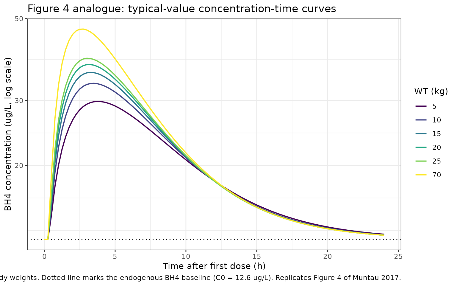

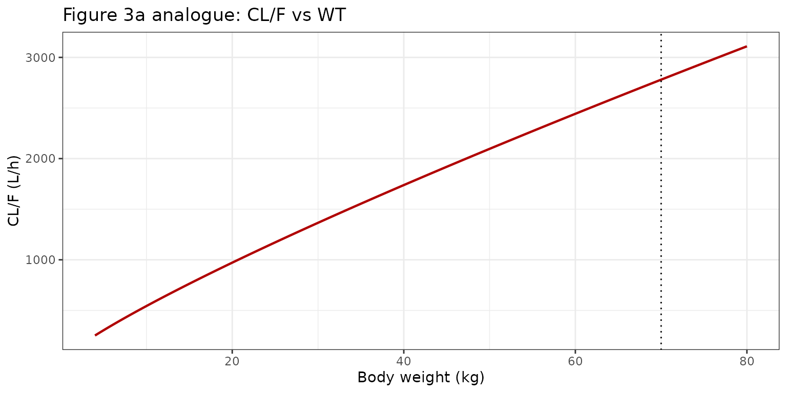
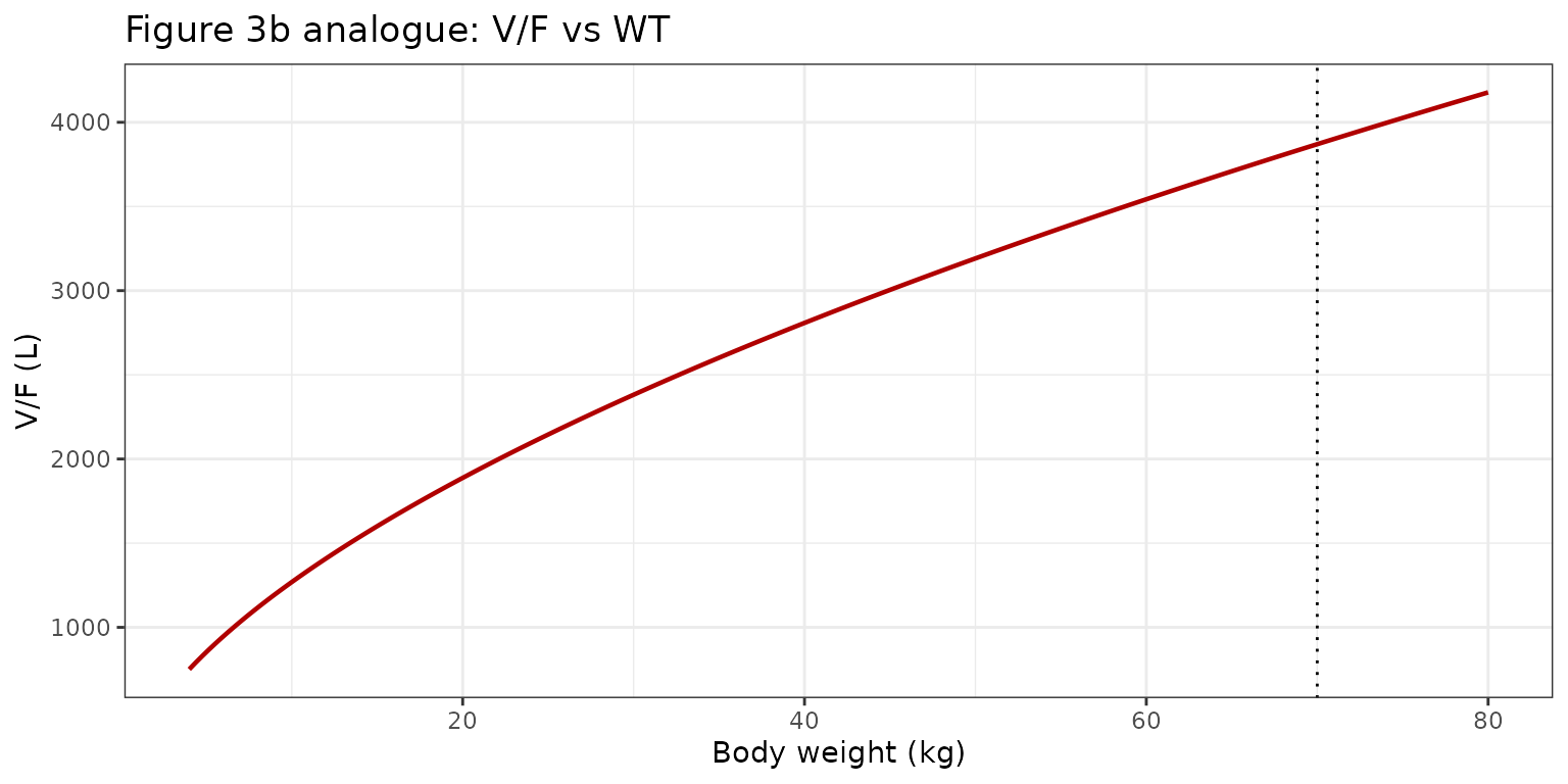
Figure 3 analogue: weight effect on CL/F and V/F

Muntau 2017 Figure 3 shows the model-implied power-form relationship between body weight and CL/F (panel a) and V/F (panel b) with the individual EBE estimates overlaid. We reproduce the typical curves analytically from the packaged thetas.

wt_grid <- seq(4, 80, length.out = 201)
cl_grid <- 2780 * (wt_grid / 70)^0.839
vc_grid <- 3870 * (wt_grid / 70)^0.573

p_cl <- ggplot(data.frame(wt = wt_grid, cl = cl_grid),
               aes(x = wt, y = cl)) +
  geom_line(colour = "#b00000", linewidth = 0.8) +
  geom_vline(xintercept = 70, linetype = "dotted") +
  labs(x = "Body weight (kg)", y = "CL/F (L/h)",
       title = "Figure 3a analogue: CL/F vs WT") +
  theme_bw()

p_vc <- ggplot(data.frame(wt = wt_grid, vc = vc_grid),
               aes(x = wt, y = vc)) +
  geom_line(colour = "#b00000", linewidth = 0.8) +
  geom_vline(xintercept = 70, linetype = "dotted") +
  labs(x = "Body weight (kg)", y = "V/F (L)",
       title = "Figure 3b analogue: V/F vs WT") +
  theme_bw()

if (requireNamespace("patchwork", quietly = TRUE)) {
  patchwork::wrap_plots(p_cl, p_vc, ncol = 2)
} else {
  print(p_cl)
  print(p_vc)
}

VPC by age stratum (SPARK trial structure)

A VPC across the three SPARK age strata at steady-state under 10 mg/kg/day dosing.

sim_vpc |>
  dplyr::filter(time_post_dose >= 0, time_post_dose <= 24) |>
  dplyr::group_by(stratum, time_post_dose) |>
  dplyr::summarise(
    Q025 = quantile(Cc, 0.025, na.rm = TRUE),
    Q50  = quantile(Cc, 0.50,  na.rm = TRUE),
    Q975 = quantile(Cc, 0.975, na.rm = TRUE),
    .groups = "drop"
  ) |>
  dplyr::mutate(stratum = factor(stratum, levels = age_strata$stratum)) |>
  ggplot(aes(x = time_post_dose, y = Q50)) +
  geom_ribbon(aes(ymin = Q025, ymax = Q975), fill = "#4682b4", alpha = 0.25) +
  geom_line(colour = "#4682b4", linewidth = 0.7) +
  geom_hline(yintercept = 12.6, linetype = "dotted") +
  facet_wrap(~ stratum) +
  scale_y_log10() +
  labs(
    x       = "Time after dose (h)",
    y       = "BH4 concentration (ug/L)",
    title   = "VPC by SPARK age stratum at steady state (10 mg/kg/day QD)",
    caption = paste0(
      "Simulated 2.5/50/97.5 percentiles by age stratum. Dotted line ",
      "marks the endogenous BH4 baseline (C0 = 12.6 ug/L)."
    )
  ) +
  theme_bw()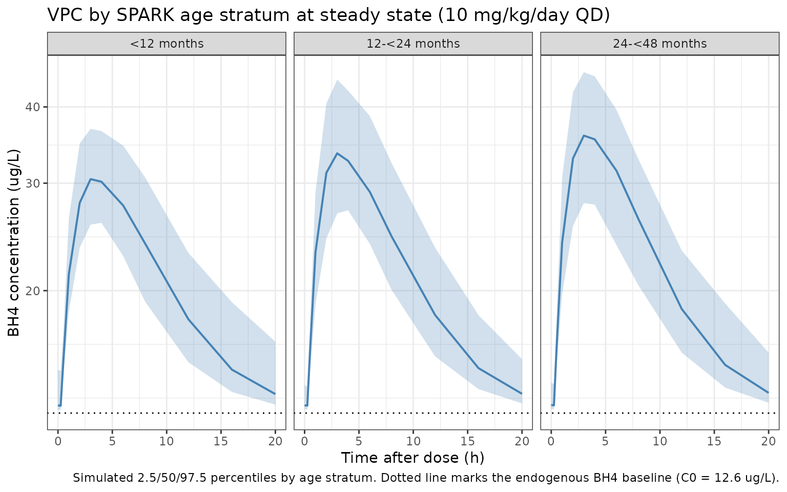

PKNCA validation

Compute NCA on simulated typical-value (no-IIV) profiles for two weights representative of the SPARK cohort (11.3 kg = SPARK mean baseline weight) and the reference adult (70 kg) given a single 10 mg/kg oral dose, sampling out to 24 hours post-dose.

obs_times_single <- c(0, 0.25, 0.5, 1, 1.5, 2, 3, 4, 5, 6,
                      8, 10, 12, 16, 20, 24, 30, 36, 48)

build_single <- function(wt, id_offset = 0L) {
  data.frame(
    ID   = id_offset + 1L,
    TIME = c(0, obs_times_single),
    AMT  = c(10 * wt, rep(0, length(obs_times_single))),
    EVID = c(1L,      rep(0L, length(obs_times_single))),
    CMT  = c("depot", rep("central", length(obs_times_single))),
    DV   = NA_real_,
    WT   = wt
  )
}

ev_single <- dplyr::bind_rows(
  build_single(11.3, id_offset = 0L)  |> dplyr::mutate(treatment = "spark_mean_11p3kg"),
  build_single(70,   id_offset = 10L) |> dplyr::mutate(treatment = "reference_70kg")
)

sim_single <- rxode2::rxSolve(mod_typical, events = ev_single,
                              keep = c("treatment")) |>
  as.data.frame()
#> ℹ omega/sigma items treated as zero: 'etalcl', 'etalvc'
#> Warning: multi-subject simulation without without 'omega'

# Subtract the endogenous baseline before NCA so Cmax / AUC / half-life
# reflect drug-derived concentrations only.
c0_value <- 12.6
sim_single <- sim_single |>
  dplyr::mutate(Cc_drug = pmax(Cc - c0_value, 0))

sim_nca <- sim_single |>
  dplyr::filter(!is.na(Cc_drug)) |>
  dplyr::transmute(id = id, time = time, Cc = Cc_drug, treatment = treatment)

dose_df <- ev_single |>
  dplyr::filter(EVID == 1) |>
  dplyr::transmute(id = ID, time = TIME, amt = AMT, treatment = treatment)

conc_obj <- PKNCA::PKNCAconc(sim_nca, Cc ~ time | treatment + id)
dose_obj <- PKNCA::PKNCAdose(dose_df, amt ~ time | treatment + id)

intervals <- data.frame(
  start      = 0,
  end        = Inf,
  cmax       = TRUE,
  tmax       = TRUE,
  aucinf.obs = TRUE,
  half.life  = TRUE
)

nca_res <- PKNCA::pk.nca(
  PKNCA::PKNCAdata(conc_obj, dose_obj, intervals = intervals)
)
knitr::kable(
  as.data.frame(nca_res$result),
  caption = paste0(
    "Single-dose drug-only NCA on the typical SPARK subject (11.3 kg) ",
    "and the reference adult (70 kg) under 10 mg/kg oral sapropterin. ",
    "Endogenous BH4 baseline (12.6 ug/L) subtracted before NCA."
  )
)

Single-dose drug-only NCA on the typical SPARK subject (11.3 kg) and the reference adult (70 kg) under 10 mg/kg oral sapropterin. Endogenous BH4 baseline (12.6 ug/L) subtracted before NCA.
treatment	id	end	PPTESTCD	PPORRES	exclude
reference_70kg	11	Inf	cmax	33.9682305	NA
reference_70kg	11	Inf	tmax	3.0000000	NA
reference_70kg	11	Inf	tlast	48.0000000	NA
reference_70kg	11	Inf	clast.obs	0.0012537	NA
reference_70kg	11	Inf	lambda.z	0.2324636	NA
reference_70kg	11	Inf	r.squared	0.9999152	NA
reference_70kg	11	Inf	adj.r.squared	0.9999058	NA
reference_70kg	11	Inf	lambda.z.time.first	5.0000000	NA
reference_70kg	11	Inf	lambda.z.time.last	48.0000000	NA
reference_70kg	11	Inf	lambda.z.n.points	11.0000000	NA
reference_70kg	11	Inf	clast.pred	0.0012843	NA
reference_70kg	11	Inf	half.life	2.9817454	NA
reference_70kg	11	Inf	span.ratio	14.4210836	NA
reference_70kg	11	Inf	aucinf.obs	250.3157275	NA
spark_mean_11p3kg	1	Inf	cmax	21.2904778	NA
spark_mean_11p3kg	1	Inf	tmax	3.0000000	NA
spark_mean_11p3kg	1	Inf	tlast	48.0000000	NA
spark_mean_11p3kg	1	Inf	clast.obs	0.0013384	NA
spark_mean_11p3kg	1	Inf	lambda.z	0.2319918	NA
spark_mean_11p3kg	1	Inf	r.squared	0.9999391	NA
spark_mean_11p3kg	1	Inf	adj.r.squared	0.9999270	NA
spark_mean_11p3kg	1	Inf	lambda.z.time.first	12.0000000	NA
spark_mean_11p3kg	1	Inf	lambda.z.time.last	48.0000000	NA
spark_mean_11p3kg	1	Inf	lambda.z.n.points	7.0000000	NA
spark_mean_11p3kg	1	Inf	clast.pred	0.0013661	NA
spark_mean_11p3kg	1	Inf	half.life	2.9878093	NA
spark_mean_11p3kg	1	Inf	span.ratio	12.0489617	NA
spark_mean_11p3kg	1	Inf	aucinf.obs	186.5912451	NA

Comparison against published half-lives

get_param <- function(res, ppname, label) {
  tbl <- as.data.frame(res$result)
  val <- tbl$PPORRES[tbl$PPTESTCD == ppname]
  lab <- tbl$treatment[tbl$PPTESTCD == ppname]
  if (length(val) == 0) return(NA_real_)
  val[match(label, lab)]
}

hl_obs_70 <- get_param(nca_res, "half.life", "reference_70kg")

# Analytical half-lives implied by the packaged thetas at WT = 70 kg
# (the reference adult, where flip-flop behavior is the source-paper claim).
ka_t   <- 0.234
cl_70  <- 2780
vc_70  <- 3870
kel_70 <- cl_70 / vc_70
hl_kel <- log(2) / kel_70    # nominal "elimination" half-life
hl_ka  <- log(2) / ka_t      # absorption half-life

comparison <- data.frame(
  Quantity = c(
    "Elimination (kel) half-life at WT = 70 kg (h)",
    "Absorption (ka) half-life (h)",
    "PKNCA terminal half-life from simulated 70 kg profile (h)"
  ),
  Published = c("~1", "~3", "(picks up rate-limiting step)"),
  Analytical = c(
    sprintf("%.2f", hl_kel),
    sprintf("%.2f", hl_ka),
    "n/a"
  ),
  Simulated = c(
    "n/a",
    "n/a",
    sprintf("%.2f", hl_obs_70)
  )
)
knitr::kable(
  comparison,
  caption = paste0(
    "Half-lives from the packaged model vs the approximate values ",
    "reported in Muntau 2017 Pharmacokinetic-analysis section ",
    "('elimination half-life of approximately 1 h ... absorption ",
    "half-life (ln2/Ka) of approximately 3 h, suggesting flip-flop ",
    "kinetics where the absorption becomes the rate-limiting step ",
    "of drug disposition'). The PKNCA terminal half-life from a ",
    "single-dose profile picks up the absorption-limited (flip-flop) ",
    "decline rather than the underlying elimination rate."
  )
)

Half-lives from the packaged model vs the approximate values reported in Muntau 2017 Pharmacokinetic-analysis section (‘elimination half-life of approximately 1 h … absorption half-life (ln2/Ka) of approximately 3 h, suggesting flip-flop kinetics where the absorption becomes the rate-limiting step of drug disposition’). The PKNCA terminal half-life from a single-dose profile picks up the absorption-limited (flip-flop) decline rather than the underlying elimination rate.
Quantity	Published	Analytical	Simulated
Elimination (kel) half-life at WT = 70 kg (h)	~1	0.96	n/a
Absorption (ka) half-life (h)	~3	2.96	n/a
PKNCA terminal half-life from simulated 70 kg profile (h)	(picks up rate-limiting step)	n/a	2.98

The analytical kel half-life (log(2) / (CL/F / V/F) = 0.96 h) reproduces the ~1 h value Muntau 2017 quotes in the Pharmacokinetic-analysis section. The analytical absorption half-life (log(2) / ka = 2.96 h) reproduces the ~3 h value the paper quotes. Because absorption is slower than elimination (ka < kel), the observed terminal-phase decline of the single-dose simulated profile is rate-limited by absorption (flip-flop PK), so the PKNCA half.life estimate tracks the absorption half-life rather than the kel half-life. This is the expected behavior the paper explicitly describes.

Assumptions and deviations

Race / ethnicity not modeled. Muntau 2017 evaluated age, weight, and sex as covariates and retained only body weight; the paper states ‘Body weight was the only covariate that affected the CL/F and V/F of sapropterin’. Race / ethnicity were not assessed as covariates in the SPARK PopPK model and are not exposed by the packaged model.
Residual error form. Table 3 reports a single residual error of 65.30% CV. The paper does not explicitly state whether the residual was log-additive (LTBS) or linear-proportional. The packaged model encodes it as proportional (Cc ~ prop(propSd)) with propSd = 0.6530, matching the standard interpretation of a reported %CV without explicit log-additive wording. For comparison, the companion Qi_2014_sapropterin model (same drug, same lead pharmacometrician D.R. Mould, broader 0-50 years cohort) used an LTBS parameterization with separate per-study residuals.
No IIV on Ka, LAG, or C0. Muntau 2017 Table 3 reports IIV only on CL/F and V/F. The packaged model leaves Ka, LAG, and C0 as typical-value (fixed-effect) parameters with no random effect, in contrast to Qi 2014 which carries IIV on C0.
Endogenous BH4 baseline added at the observation step. Following the same convention as Qi 2014, the packaged model adds c0 = 12.6 ug/L as a constant offset on the predicted plasma concentration rather than modeling its synthesis / clearance dynamics. For NCA validation in this vignette, the endogenous baseline is subtracted before PKNCA so that Cmax / AUC reflect drug-derived exposure (the paper’s narrative refers to BH4 concentrations ‘above the model-estimated endogenous BH4 concentrations’).
Flip-flop kinetics. Because absorption (ka = 0.234 h^-1 -> absorption half-life ~3 h) is slower than nominal elimination (kel = CL/F divided by V/F = 0.718 h^-1 at 70 kg -> elimination half-life ~1 h), the observed terminal-phase log-linear decline reflects absorption, not elimination, as Muntau 2017 explicitly notes. PKNCA half.life therefore returns ~3 h (absorption half-life) rather than ~1 h (elimination half-life); the analytical kel value is reported alongside for comparison.
Virtual cohort weight distributions. Exact baseline weight distributions per age stratum are not published; the vignette uses truncated normal weight draws whose mean / range match Table 2 and the age-stratum counts reported in ‘Patient disposition and demographics’.
No bioavailability parameter exposed. Sapropterin is administered orally and the original analysis reports apparent parameters (CL/F and V/F). The packaged model uses the same apparent parameterization and does not declare a separate lfdepot – bioavailability is implicit and not separately identifiable.
Reference weight. Table 4 footnote ‘a Reference weight (adult male patient)’ identifies 70 kg as the reference for the power-form normalization. The packaged model uses (WT / 70)^e_wt_* for both CL/F and V/F.

Reference

Muntau AC, Burlina A, Eyskens F, et al. Efficacy, safety and population pharmacokinetics of sapropterin in PKU patients <4 years: results from the SPARK open-label, multicentre, randomized phase IIIb trial. Orphanet Journal of Rare Diseases. 2017;12:47. doi:10.1186/s13023-017-0600-x