Vancomycin (Avachat 2025)
Source:vignettes/articles/Avachat_2025_vancomycin.Rmd
Avachat_2025_vancomycin.RmdModel and source
- Citation: Avachat C, Hung CC, Birnbaum AK, Healy DP, Sherwin CMT, Lin YC. Pharmacokinetic effect of disease severity and use of extracorporeal membrane oxygenation in critically ill Asian patients receiving vancomycin. Front Pharmacol. 2025;16:1506793. doi:10.3389/fphar.2025.1506793. PMID 40078297; PMCID PMC11897554.
- Description: One-compartment IV population PK model for vancomycin in critically ill, predominantly paediatric Asian patients (Taiwan; age 0.1-36.6 years, weight 0.7-93 kg) receiving therapeutic drug monitoring (Avachat 2025). Clearance scales allometrically with body weight (exponent fixed at 0.75) and volume linearly (exponent fixed at 1), both normalised to the 12.6 kg cohort median; clearance is further reduced by exp(-0.81) (about 56%) in patients on extracorporeal membrane oxygenation (ECMO) and by exp(-0.49) (about 39%) in patients whose vancomycin indication was a milder infection (cellulitis, surgical prophylaxis, neutropenic fever or other) rather than a severe one (pneumonia, bacteremia, osteomyelitis, meningitis or deep tissue infection). Exponential between-subject variability on CL and V; proportional residual error.
- Article: https://doi.org/10.3389/fphar.2025.1506793
- Open-access copy: https://www.ncbi.nlm.nih.gov/pmc/articles/PMC11897554/
Population
Avachat 2025 is a retrospective analysis of therapeutic drug monitoring (TDM) data from 90 critically ill patients treated with intravenous vancomycin at Kaohsiung Veterans General Hospital, Taiwan, between 2014 and 2016 (Table 1). Ninety percent were children: median age 3.7 years (range 0.1 to 36.6) and median weight 12.6 kg (range 0.7 to 93). There were 47 males and 43 females. Median eGFR (bedside Schwartz) was 70.4 (range 2.4 to 150.6); one patient was on regular haemodialysis and one on CRRT. Twelve patients (13.3%) were on extracorporeal membrane oxygenation (ECMO) and 33 (36.7%) had surgery.
The authors grouped the nine admission diagnoses by the severity of the infection for which vancomycin was given: severe = pneumonia (20), bacteremia (6), osteomyelitis (7), meningitis (4) and deep tissue infection (1), 38 patients; mild = cellulitis (6), surgical prevention (35), neutropenic fever (4) and others (7), 52 patients. The 263 concentrations were mostly troughs (drawn within 30 min before a dose), with some peaks (> 1 h after the end of infusion). The model was fitted in Phoenix NLME 8.2 with FOCE-ELS.
The same information is available programmatically via
readModelDb("Avachat_2025_vancomycin")()$population.
Source trace
| Equation / parameter | Value | Source location |
|---|---|---|
lcl = log(1.03) |
1.03 L/h | Table 4, tvCL (L/h) (SE 0.099, 95% CI 0.84-1.23) |
lvc = log(11.61) |
11.61 L | Table 4, tvV (L) (SE 1.22, 95% CI 9.2-14.03) |
e_wt_cl |
0.75 (fixed) | Table 4, dCldWT (fixed); Section 2.2 |
e_wt_vc |
1 (fixed) | Table 4, dVdWT (fixed); Section 2.2 |
e_ecmo_status_cl |
-0.81 | Table 4, dCldECMO (SE 0.17, 95% CI -1.14 to -0.47) |
e_infect_mild_cl |
-0.49 | Table 4, dCldDiag (SE 0.18, 95% CI -0.84 to -0.14) |
etalcl |
0.26 (variance) | Table 4, eta Cl (SE 0.08, shrinkage 0.27) |
etalvc |
0.24 (variance) | Table 4, eta V (SE 0.07, shrinkage 0.52) |
propSd |
0.44 | Table 4, Stdev0 (SE 0.03); Section 3.2 proportional
error |
| Reference weight 12.6 kg | n/a | Section 3.3 equations (WT/median(WT)) and the following
paragraph; Table 1 median |
cl equation |
n/a | Section 3.3, first final-model equation |
vc equation |
n/a | Section 3.3, second final-model equation |
| One compartment, first-order elimination | n/a | Section 3.2 |
Verification against the published worked example
Table 3 of the paper substitutes the final estimates into the clearance equation for a 12.6 kg patient with no random effect. The packaged model, solved with the random effects removed, must reproduce it.
mod <- readModelDb("Avachat_2025_vancomycin")

tab3 <- tibble::tibble(
  id              = 1:4,
  group           = c("No ECMO, severe infection", "ECMO, severe infection",
                      "No ECMO, mild infection", "ECMO, mild infection"),
  ECMO_STATUS     = c(0, 1, 0, 1),
  DIS_INFECT_MILD = c(0, 0, 1, 1),
  # Table 3 'Clearance value (L/h)'; the paper does not tabulate the
  # combined ECMO + mild group.
  cl_paper        = c(1.03, 0.48, 0.63, NA),
  pct_paper       = c(NA, 56, 39, NA)
)

typ_ev <- tab3 |>
  select(id, ECMO_STATUS, DIS_INFECT_MILD) |>
  mutate(WT = 12.6) |>
  tidyr::crossing(time = c(0, 1)) |>
  mutate(evid = 0L, cmt = "central", amt = NA_real_)

typ <- rxode2::rxSolve(rxode2::zeroRe(mod), events = typ_ev) |>
  as.data.frame() |>
  group_by(id) |>
  summarise(cl = first(cl), vc = first(vc), .groups = "drop") |>
  left_join(tab3, by = "id") |>
  mutate(pct_reduction = 100 * (1 - cl / cl[1]))
#> ℹ parameter labels from comments will be replaced by 'label()'
#> ℹ omega/sigma items treated as zero: 'etalcl', 'etalvc'
#> Warning: multi-subject simulation without without 'omega'

typ |>
  select(group, cl, cl_paper, pct_reduction, pct_paper, vc) |>
  rename(
    "Group"                       = group,
    "CL, model (L/h)"             = cl,
    "CL, Table 3 (L/h)"           = cl_paper,
    "CL reduction, model (%)"     = pct_reduction,
    "CL reduction, paper (%)"     = pct_paper,
    "V, model (L)"                = vc
  ) |>
  knitr::kable(
    digits  = 3,
    caption = "Typical clearance at the 12.6 kg reference weight, against Avachat 2025 Table 3."
)| Group | CL, model (L/h) | CL, Table 3 (L/h) | CL reduction, model (%) | CL reduction, paper (%) | V, model (L) |
|---|---|---|---|---|---|
| No ECMO, severe infection | 1.030 | 1.03 | 0.000 | NA | 11.61 |
| ECMO, severe infection | 0.458 | 0.48 | 55.514 | 56 | 11.61 |
| No ECMO, mild infection | 0.631 | 0.63 | 38.737 | 39 | 11.61 |
| ECMO, mild infection | 0.281 | NA | 72.747 | NA | 11.61 |
# Deterministic arithmetic: no random effects on either side.
stopifnot(
  abs(typ$cl[1] - 1.03) < 1e-8,
  abs(typ$vc[1] - 11.61) < 1e-8,
  abs(typ$cl[3] - 0.63) < 0.005,
  abs(typ$pct_reduction[2] - 56) < 1,
  abs(typ$pct_reduction[3] - 39) < 1
)
The model reproduces the reference clearance, the mild-infection
clearance (0.631 L/h against the printed 0.63) and both percentage
reductions (55.5% and 38.7%, printed as about 56% and 39%). Table 3 and
the Results text print the ECMO clearance as 0.48 L/h, but the
substitution the table itself writes out,
1.03 * 1^0.75 * exp(-0.81), evaluates to 0.458 L/h; the
printed 0.48 does not follow from the printed estimates, while the
printed 56% reduction does. The model uses the Table 4 estimate of
-0.81.
Typical elimination half-life for a 12.6 kg patient with a severe
infection and no ECMO is log(2) * 11.61 / 1.03 = 7.8 h.
Virtual cohort
Individual data are not published. The cohort below draws body weight from a log-normal distribution with the cohort median of 12.6 kg, truncated to the observed 0.7 to 93 kg range. The paper reports no dosing regimen (only that infusion rates ranged from 8 to 1500 mg/h), so every subject receives 15 mg/kg every 6 h as a 1-h infusion (60 mg/kg/day), a common paediatric starting regimen. This is an assumption of the vignette.
Each of the four covariate groups (ECMO yes/no by severe/mild
infection) gets 100 subjects with identical weight draws, so the groups
differ only by the covariate effects and the random effects.
Concentrations are simulated at steady state with ss = 1,
over one dosing interval.
# set.seed() fixes the weight draws. rxode2's own random-effect draws are not
# reproducible across rxode2 builds or thread counts, so the assertions below
# compare each subject with itself or with closed forms.
set.seed(20251306)

n_per_group <- 100L
tau         <- 6
infusion_h  <- 1

draw_trunc_lnorm <- function(n, median_value, sdlog, lower, upper) {
  out <- numeric(0)
  while (length(out) < n) {
    cand <- stats::rlnorm(n * 3L, log(median_value), sdlog)
    out <- c(out, cand[cand >= lower & cand <= upper])
  }
  out[seq_len(n)]
}

weights <- draw_trunc_lnorm(n_per_group, 12.6, 1.1, 0.7, 93)

groups <- tab3 |>
  select(group, ECMO_STATUS, DIS_INFECT_MILD) |>
  mutate(group_index = seq_len(n()))

subjects <- groups |>
  tidyr::expand_grid(subject = seq_len(n_per_group)) |>
  mutate(
    id  = (group_index - 1L) * n_per_group + subject,
    WT  = weights[subject],
    amt = 15 * WT
  )

doses <- subjects |>
  mutate(
    time = 0, evid = 1L, cmt = "central",
    rate = amt / infusion_h, ss = 1L, ii = tau
  )

# Observation rows reference the ODE state, never the observable Cc.
obs <- subjects |>
  tidyr::expand_grid(time = seq(0, tau, by = 0.05)) |>
  mutate(
    evid = 0L, cmt = "central", amt = NA_real_,
    rate = NA_real_, ss = NA_integer_, ii = NA_real_
  )

events <- bind_rows(doses, obs) |>
  arrange(id, time, desc(evid)) |>
  select(id, time, amt, evid, cmt, rate, ss, ii, WT, ECMO_STATUS,
         DIS_INFECT_MILD, group)

stopifnot(length(unique(events$id)) == 4L * n_per_group)

cat(sprintf(
  "Weights: median %.1f kg (range %.1f-%.1f)\n",
  median(weights), min(weights), max(weights)
))
#> Weights: median 10.7 kg (range 1.2-91.7)Steady-state profiles by covariate group
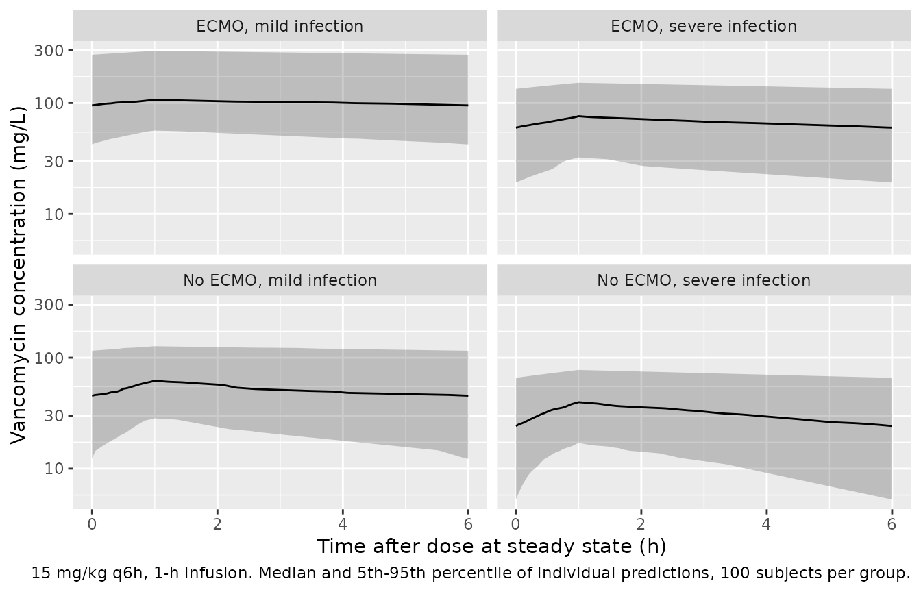
Figure 3 of the paper is a visual predictive check against time since the first dose (up to about 8000 h) for the observed regimens, which are not published, so it cannot be redrawn. The plot below shows the steady-state interval for the assumed regimen in each covariate group, on the same logarithmic concentration axis.
sim |>
  filter(!is.na(Cc)) |>
  group_by(group, time) |>
  summarise(
    Q05 = quantile(Cc, 0.05),
    Q50 = quantile(Cc, 0.50),
    Q95 = quantile(Cc, 0.95),
    .groups = "drop"
  ) |>
  ggplot(aes(time, Q50)) +
  geom_ribbon(aes(ymin = Q05, ymax = Q95), alpha = 0.25) +
  geom_line() +
  facet_wrap(~group) +
  scale_y_log10() +
  labs(
    x = "Time after dose at steady state (h)",
    y = "Vancomycin concentration (mg/L)",
    caption = "15 mg/kg q6h, 1-h infusion. Median and 5th-95th percentile of individual predictions, 100 subjects per group."
  )
PKNCA validation
sim_nca <- sim |>
  filter(!is.na(Cc)) |>
  select(id, time, Cc, group)

conc_obj <- PKNCA::PKNCAconc(
  sim_nca, Cc ~ time | group + id,
  concu = "mg/L", timeu = "h"
)

dose_df <- events |>
  filter(evid == 1) |>
  select(id, time, amt, group)

dose_obj <- PKNCA::PKNCAdose(
  dose_df, amt ~ time | group + id,
  doseu = "mg"
)

intervals <- data.frame(
  start   = 0,
  end     = tau,
  auclast = TRUE,
  cmax    = TRUE,
  cmin    = TRUE
)

nca_res <- PKNCA::pk.nca(PKNCA::PKNCAdata(conc_obj, dose_obj, intervals = intervals))

nca_wide <- as.data.frame(nca_res) |>
  select(group, id, PPTESTCD, PPORRES) |>
  tidyr::pivot_wider(names_from = PPTESTCD, values_from = PPORRES)

nca_wide |>
  group_by(group) |>
  summarise(
    cmax    = median(cmax),
    cmin    = median(cmin),
    auclast = median(auclast),
    .groups = "drop"
  ) |>
  rename(
    "Group"                      = group,
    "Median Cmax,ss (mg/L)"      = cmax,
    "Median Cmin,ss (mg/L)"      = cmin,
    "Median AUC0-6,ss (mg*h/L)"  = auclast
  ) |>
knitr::kable(digits = 1, caption = "Steady-state NCA by covariate group, 15 mg/kg q6h.")| Group | Median Cmax,ss (mg/L) | Median Cmin,ss (mg/L) | Median AUC0-6,ss (mg*h/L) |
|---|---|---|---|
| ECMO, mild infection | 107.2 | 95.2 | 609.0 |
| ECMO, severe infection | 76.2 | 60.0 | 401.1 |
| No ECMO, mild infection | 62.1 | 45.4 | 301.3 |
| No ECMO, severe infection | 39.7 | 24.2 | 188.7 |
Mass balance: steady-state AUC over one interval equals Dose/CL
For a linear model the steady-state AUC over one dosing interval
equals Dose / CL for each subject. Both sides use the same
simulated individual clearance, so the only difference is trapezoidal
error on the 0.05 h grid and a tight bound is right.
mb <- nca_wide |>
  left_join(
    sim |> group_by(id) |> summarise(cl = first(cl), WT = first(WT), .groups = "drop"),
    by = "id"
  ) |>
  mutate(ratio = auclast / (15 * WT / cl))

tibble(
  Subjects          = nrow(mb),
  `Max |ratio - 1|` = max(abs(mb$ratio - 1))
) |>
knitr::kable(digits = 6, caption = "PKNCA AUC0-tau at steady state against Dose/CL.")| Subjects | Max |ratio - 1| |
|---|---|
| 400 | 6e-05 |
Group contrasts
The median steady-state AUC ratio between groups is the clearance ratio: exp(-0.81) = 0.445 for ECMO and exp(-0.49) = 0.613 for a mild infection, so AUC rises 2.25-fold on ECMO and 1.63-fold for a mild infection. Because the groups share weight draws but not random effects, the comparison is on medians.
auc_med <- nca_wide |>
  group_by(group) |>
  summarise(auc = median(auclast), .groups = "drop")

ref_auc <- auc_med$auc[auc_med$group == "No ECMO, severe infection"]

contrast <- auc_med |>
  mutate(
    ratio_sim      = auc / ref_auc,
    ratio_expected = c(
      "No ECMO, severe infection" = 1,
      "ECMO, severe infection"    = exp(0.81),
      "No ECMO, mild infection"   = exp(0.49),
      "ECMO, mild infection"      = exp(0.81 + 0.49)
    )[group],
    pct_diff = 100 * (ratio_sim / ratio_expected - 1)
  )

contrast |>
  rename(
    "Group"                       = group,
    "Median AUC0-6,ss (mg*h/L)"   = auc,
    "AUC ratio, simulated"        = ratio_sim,
    "AUC ratio, 1/CL multiplier"  = ratio_expected,
    "% difference"                = pct_diff
  ) |>
knitr::kable(digits = 2, caption = "Median steady-state AUC relative to the reference group.")| Group | Median AUC0-6,ss (mg*h/L) | AUC ratio, simulated | AUC ratio, 1/CL multiplier | % difference |
|---|---|---|---|---|
| ECMO, mild infection | 609.00 | 3.23 | 3.67 | -12.03 |
| ECMO, severe infection | 401.12 | 2.13 | 2.25 | -5.43 |
| No ECMO, mild infection | 301.28 | 1.60 | 1.63 | -2.18 |
| No ECMO, severe infection | 188.68 | 1.00 | 1.00 | 0.00 |
Assumptions and deviations
-
Omega scale. Table 4 lists
eta Cl= 0.26 andeta V= 0.24 without stating whether these are variances or standard deviations. Phoenix NLME reports the Omega matrix as variances, so they are used as variances (lognormal CV about 54% and 52%). The paper’s%CVcolumn beside them is the relative standard error of the estimate (0.08 / 0.26 = 30.7%), not the between-subject CV. -
Residual error. Section 3.2 selects a proportional
error model and Section 5 describes “a relatively high residual error of
44%”; Table 4’s
Stdev0= 0.44 is therefore the proportional SD. Section 2.2 mentions natural-log transformed concentrations, which the text ties to the plotting of the data; the error model is taken as proportional, as the Results state. - ECMO clearance printed as 0.48 L/h. The printed estimates give 0.458 L/h (see the Table 3 check above); the model uses the Table 4 coefficient.
-
Reference weight. The equations print
WT/median(WT); the 12.6 kg median is stated in the text and Table 1. - ECMO and infection category are subject-level. The paper gives no within-subject timing for ECMO cannulation; diagnosis is the admission diagnosis.
- Covariates not retained. Surgery status (removed at backward elimination, Table 2) and eGFR (not significant) are not in the model.
- Dosing regimen. The paper does not report individual regimens; the 15 mg/kg q6h, 1-h infusion regimen used here is illustrative.
- No published NCA. The paper reports no Cmax, AUC or half-life values, so there is no NCA comparison table; the checks above are against the paper’s own Table 3 arithmetic and against closed forms.