Dalteparin (Damle 2021)

Model and source

• Citation: Damle B, Jen F, Sherman N, Jani D, Sweeney K. Population Pharmacokinetic Analysis of Dalteparin in Pediatric Patients With Venous Thromboembolism. J Clin Pharmacol. 2021;61(2):172-180. doi:10.1002/jcph.1716
• Description: One-compartment population PK model with first-order absorption and elimination for subcutaneous dalteparin in pediatric patients (1 month to 19 years) with venous thromboembolism, fitted to plasma anti-factor Xa activity as the surrogate concentration (Damle 2021 full covariate model). CL/F and V/F scale allometrically with body weight (exponents fixed at 0.75 and 1, reference 43 kg); CL/F additionally has a power effect of age (reference 12 years) and multiplicative male-sex and no-cancer factors (reference: a female patient with cancer). The IIV of V/F is the IIV of CL/F multiplied by an estimated scaling factor (perfect correlation); combined proportional plus additive residual error.
• Article: https://doi.org/10.1002/jcph.1716 (open access)

Dalteparin is a low-molecular-weight heparin. Because the drug itself is difficult to assay, its pharmacokinetics are described through plasma anti-factor Xa (anti-Xa) activity, so the model’s “concentration” Cc is anti-Xa activity in IU/mL and doses are in anti-Xa IU.

Population

Damle 2021 pooled 266 anti-Xa observations from 89 pediatric patients with acute venous thromboembolism (VTE) from three sources: a Pfizer-sponsored prospective open-label study (NCT00952380, 15 sites in North America and Europe, n = 37), the dose-finding pilot of the Kids-DOTT trial (n = 18) and a Mayo Clinic retrospective chart review (n = 34). Age ranged from 15 days to 19.5 years (median 12.0 years), body weight from 2.3 to 161 kg (median 43.4 kg); 66.3% were male, 45% were white and 48.3% had cancer (Table 1). Patients received subcutaneous dalteparin twice daily, starting at 100-150 IU/kg by age group and titrated to a 4-6 h post-dose anti-Xa target of 0.5-1.0 IU/mL; most samples were drawn 3-6 h after a dose.

str(rxode2::rxode2(readModelDb("Damle_2021_dalteparin"))$population)
#> ℹ parameter labels from comments will be replaced by 'label()'
#> List of 15
#>  $ species       : chr "human"
#>  $ n_subjects    : int 89
#>  $ n_studies     : int 3
#>  $ n_observations: int 266
#>  $ age_range     : chr "0.04-19.5 years (15 days to 19.5 years)"
#>  $ age_median    : chr "12.0 years"
#>  $ weight_range  : chr "2.3-161 kg"
#>  $ weight_median : chr "43.4 kg"
#>  $ sex_female_pct: num 33.7
#>  $ race_ethnicity: Named num 45
#>   ..- attr(*, "names")= chr "White"
#>  $ disease_state : chr "Pediatric patients with acute venous thromboembolism requiring therapeutic anticoagulation, with (48.3%) or without cancer."
#>  $ dose_range    : chr "Subcutaneous dalteparin twice daily, starting doses 100-150 IU/kg by age group, titrated in 25 IU/kg steps (or "| __truncated__
#>  $ regions       : chr "North America and Europe (15 sites in the Pfizer study NCT00952380), plus the multicenter Kids-DOTT pilot and a"| __truncated__
#>  $ age_groups    : chr "0 to <8 weeks n = 6; 8 weeks to <2 years n = 13; 2 to <8 years n = 14; 8 to <12 years n = 11; 12 to <19 years n"| __truncated__
#>  $ notes         : chr "Pooled from the Pfizer-sponsored open-label study (n = 37), the Kids-DOTT dose-finding pilot (n = 18) and a May"| __truncated__

Source trace

Model element	Value	Source location
Structure: 1-compartment, first-order absorption and elimination, parameterised in CL/F, V/F, ka	-	Results, Population Pharmacokinetic Analysis
lcl (CL/F, 43 kg, 12 y, female, with cancer)	929 mL/h = 0.929 L/h	Table 2, theta1
lvc (V/F, 43 kg)	7180 mL = 7.18 L	Table 2, theta2
lka	1.04 1/h	Table 2, theta3
vc_eta_scale	1.73	Table 2, theta5; equation eta_V = theta5 * eta_CL
e_wt_cl	0.75 (fixed)	Table 2, theta6; Methods
e_wt_vc	1 (fixed)	Table 2, theta7; Methods
e_age_cl	-0.0687	Table 2, theta8
e_sexm_cl	1.03 (male)	Table 2, theta14
e_nocancer_cl	0.885 (without cancer)	Table 2, theta15
etalcl	0.0369 (19% CV)	Table 2, omega2 CL/F
propSd	sqrt(0.0519) = 0.228	Table 2, sigma2 P (text: 23% CV)
addSd	sqrt(0.016) = 0.1265 IU/mL	Table 2, sigma2 A
TVCL = theta1 (WT/43)^theta6 (AGE/12)^theta8 theta14^I(male) theta15^I(no cancer)	-	Results, model equations (page 175)
TVV = theta2 (WT/43)^theta7	-	Results, model equations (page 175)

Virtual cohort

The paper simulated 1000 subjects per age group “based on the age-weight relationship in the current population pharmacokinetic data set”, which is not published. Here age is drawn uniformly within each of the paper’s five age groups, and body weight is drawn log-normally (20% CV) around a weight-age curve interpolated through the per-group median ages and weights of Table 1. Each group has 200 subjects. The between-subject random effect etalcl is drawn with base R and passed to the model as a data column, so the cohort does not depend on the rxode2 random-number stream and the checks below are deterministic.

mod <- rxode2::rxode2(readModelDb("Damle_2021_dalteparin"))
#> ℹ parameter labels from comments will be replaced by 'label()'
omega_cl <- mod$omega["etalcl", "etalcl"]
prop_sd <- mod$theta[["propSd"]]
add_sd <- mod$theta[["addSd"]]

# Table 1 per-group median age (years) and weight (kg)
anchor <- data.frame(
  age = c(0.06, 0.5, 4.5, 9.6, 15.9),
  wt = c(3.5, 6.8, 14.6, 36.1, 61.8)
)
median_wt <- function(age) stats::approx(anchor$age, anchor$wt, xout = age, rule = 2)$y

groups <- data.frame(
  group = c(
    "0 to <8 weeks", ">=8 weeks to <2 years", ">=2 to <8 years",
    ">=8 to <12 years", ">=12 to <19 years"
  ),
  age_lo = c(15 / 365.25, 8 / 52, 2, 8, 12),
  age_hi = c(8 / 52, 2, 8, 12, 19)
)
groups$group <- factor(groups$group, levels = groups$group)

n_per_group <- 200L # cohort cap: never more than 200 participants per arm
set.seed(20210201)
cohort <- bind_rows(lapply(seq_len(nrow(groups)), function(i) {
  age <- stats::runif(n_per_group, groups$age_lo[i], groups$age_hi[i])
  data.frame(
    group = groups$group[i],
    AGE = age,
    WT = median_wt(age) * exp(stats::rnorm(n_per_group, 0, 0.2)),
    etalcl = stats::rnorm(n_per_group, 0, sqrt(omega_cl))
  )
})) |>
  mutate(
    id = row_number(),
    # The paper's dose simulations used a reduced model without the sex and
    # cancer factors; with theta14 = theta15 = 1 dropped that is the full model
    # at its reference levels (female, with cancer).
    SEXF = 1,
    DIS_CANCER_PED = 1
  )

cohort |>
  group_by(group) |>
  summarise(
    n = n(),
    `Age median (y)` = signif(median(AGE), 3),
    `WT median (kg)` = signif(median(WT), 3),
    `WT range (kg)` = paste(signif(range(WT), 3), collapse = "-")
  ) |>
  knitr::kable()

group	n	Age median (y)	WT median (kg)	WT range (kg)
0 to <8 weeks	200	0.0992	3.85	2.05-6.31
>=8 weeks to <2 years	200	1.0300	7.89	3.69-14.9
>=2 to <8 years	200	4.6800	16.70	7.27-35.1
>=8 to <12 years	200	10.1000	38.00	21.3-74.4
>=12 to <19 years	200	15.3000	55.80	26.8-136

Simulation

Steady-state twice-daily (every 12 h) dosing is simulated with ss = 1, and observations are taken on the central state. The model is solved with its random effects zeroed (rxode2::zeroRe()) because the per-subject etalcl comes from the data; the residual error is then applied analytically below.

mod_typ <- rxode2::zeroRe(mod)

# The random-effect variances are zeroed on purpose, so the "simulation
# without omega" warning is expected and muffled; any other warning surfaces.
solve_ss <- function(events) {
  withCallingHandlers(
    rxode2::rxSolve(mod_typ, events, returnType = "data.frame", keep = "group"),
    warning = function(w) {
      if (grepl("without 'omega'", conditionMessage(w), fixed = TRUE)) {
        invokeRestart("muffleWarning")
      }
    }
  )
}

make_events <- function(cohort, dose_per_kg, obs_times) {
  dose_rows <- cohort |>
    mutate(
      time = 0, amt = dose_per_kg * WT, evid = 1L, cmt = "depot",
      ss = 1L, ii = 12
    )
  obs_rows <- tidyr::crossing(cohort, time = obs_times) |>
    mutate(amt = 0, evid = 0L, cmt = "central", ss = 0L, ii = 0)
  bind_rows(dose_rows, obs_rows) |>
    arrange(id, time, desc(evid))
}

Probability of target attainment (Figure 4)

For each age group and each dose from 75 to 300 IU/kg every 12 h, the steady-state anti-Xa level 4 h after a dose (C4hss) is computed. The probabilities of target attainment (0.5-1.0 IU/mL), underattainment and overattainment then integrate the combined residual error of the model over each subject’s individual prediction: an observation is normal around the prediction with SD sqrt(addSd^2 + (propSd * pred)^2). Including the residual error is what reproduces the paper’s figure. Using the individual prediction alone gives maximum PTAs near 0.85, where the paper reports 0.61-0.66.

doses <- seq(75, 300, by = 25)
c4 <- bind_rows(lapply(doses, function(d) {
  solve_ss(make_events(cohort, d, obs_times = 4)) |>
    filter(time == 4) |>
    transmute(id, group, dose = d, pred = Cc)
}))
#> ℹ omega/sigma items treated as zero: 'etalcl'
#> ℹ omega/sigma items treated as zero: 'etalcl'
#> ℹ omega/sigma items treated as zero: 'etalcl'
#> ℹ omega/sigma items treated as zero: 'etalcl'
#> ℹ omega/sigma items treated as zero: 'etalcl'
#> ℹ omega/sigma items treated as zero: 'etalcl'
#> ℹ omega/sigma items treated as zero: 'etalcl'
#> ℹ omega/sigma items treated as zero: 'etalcl'
#> ℹ omega/sigma items treated as zero: 'etalcl'
#> ℹ omega/sigma items treated as zero: 'etalcl'

pta <- c4 |>
  mutate(
    sd = sqrt(add_sd^2 + (prop_sd * pred)^2),
    p_under = stats::pnorm(0.5, pred, sd),
    p_over = 1 - stats::pnorm(1, pred, sd)
  ) |>
  group_by(group, dose) |>
  summarise(
    under = mean(p_under),
    over = mean(p_over),
    .groups = "drop"
  ) |>
  mutate(pta = 1 - under - over)

Values digitised by the maintainers from Figure 4 of Damle 2021 (read to about +/-0.02) are overlaid as points.

fig4 <- tibble::tibble(
  group = rep(levels(groups$group), each = length(doses)),
  dose = rep(doses, times = 5),
  pta = c(
    0.01, 0.04, 0.11, 0.20, 0.30, 0.45, 0.56, 0.61, 0.66, 0.66,
    0.07, 0.18, 0.33, 0.49, 0.58, 0.64, 0.62, 0.61, 0.55, 0.47,
    0.15, 0.33, 0.52, 0.63, 0.64, 0.61, 0.51, 0.40, 0.33, 0.25,
    0.27, 0.53, 0.61, 0.60, 0.54, 0.44, 0.33, 0.25, 0.15, 0.12,
    0.32, 0.54, 0.64, 0.58, 0.48, 0.36, 0.27, 0.17, 0.13, 0.09
  ),
  over = c(
    0.00, 0.00, 0.00, 0.00, 0.005, 0.01, 0.02, 0.04, 0.10, 0.15,
    0.00, 0.00, 0.005, 0.02, 0.06, 0.10, 0.20, 0.27, 0.38, 0.48,
    0.00, 0.00, 0.03, 0.09, 0.18, 0.30, 0.46, 0.55, 0.65, 0.73,
    0.005, 0.02, 0.10, 0.24, 0.38, 0.51, 0.64, 0.74, 0.84, 0.87,
    0.01, 0.05, 0.13, 0.30, 0.46, 0.61, 0.72, 0.82, 0.86, 0.91
  )
) |>
  mutate(group = factor(group, levels = levels(groups$group)))

pta_long <- pta |>
  select(group, dose, `Target (0.5-1.0 IU/mL)` = pta, `Over (>1.0 IU/mL)` = over, `Under (<0.5 IU/mL)` = under) |>
  pivot_longer(-c(group, dose), names_to = "outcome", values_to = "probability")
fig4_long <- fig4 |>
  select(group, dose, `Target (0.5-1.0 IU/mL)` = pta, `Over (>1.0 IU/mL)` = over) |>
  pivot_longer(-c(group, dose), names_to = "outcome", values_to = "probability")

ggplot(pta_long, aes(dose, probability, colour = outcome)) +
  geom_line(linewidth = 0.9) +
  geom_point(data = fig4_long, shape = 1, size = 2) +
  geom_hline(yintercept = 0.5, linetype = "dashed", colour = "grey50") +
  facet_wrap(~group) +
  scale_colour_manual(values = c(
    "Target (0.5-1.0 IU/mL)" = "forestgreen",
    "Over (>1.0 IU/mL)" = "red3", "Under (<0.5 IU/mL)" = "orange"
  )) +
  labs(
    x = "Dalteparin dose every 12 h (IU/kg)", y = "Probability",
    colour = NULL,
    caption = "Replicates Figure 4 of Damle 2021. Lines: this model; open points: digitised from the paper."
  ) +
  theme_bw() +
  theme(legend.position = "bottom")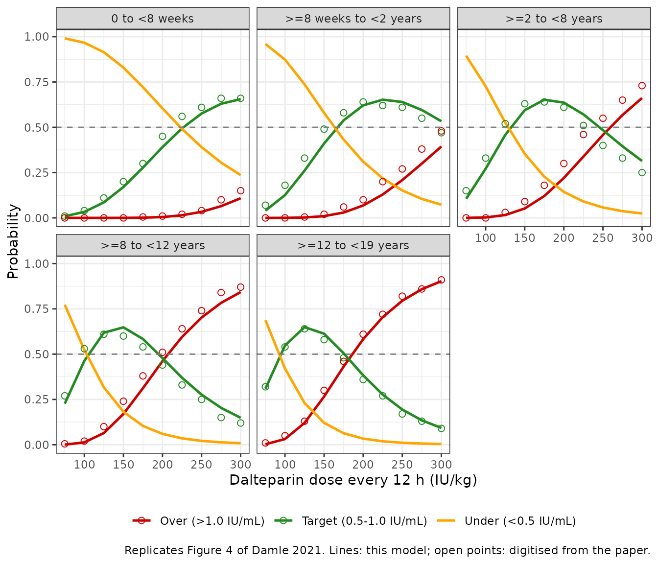

The dose at which the rising PTA curve crosses 0.5 is the paper’s criterion for the starting dose (dashed lines in its Figure 4; the paper rounds these to 200, 150, 125, 100 and 100 IU/kg).

dose_at_half <- function(dose, p) {
  i <- which(p >= 0.5)[1]
  stats::approx(p[(i - 1):i], dose[(i - 1):i], xout = 0.5)$y
}
pta_summary <- pta |>
  group_by(group) |>
  summarise(
    dose50 = dose_at_half(dose, pta),
    max_pta = max(pta),
    .groups = "drop"
  ) |>
  mutate(
    paper_dose50 = c(210, 155, 122, 97, 95),
    paper_max_pta = fig4 |> group_by(group) |> summarise(m = max(pta)) |> pull(m),
    dose50_pct_diff = 100 * (dose50 - paper_dose50) / paper_dose50
  )
pta_summary |>
  mutate(across(where(is.numeric), ~ signif(.x, 3))) |>
  rename(
    `Age group` = group,
    `Dose at 50% PTA, model (IU/kg)` = dose50,
    `Max PTA, model` = max_pta,
    `Dose at 50% PTA, Figure 4 (IU/kg)` = paper_dose50,
    `Max PTA, Figure 4` = paper_max_pta,
    `Dose difference (%)` = dose50_pct_diff
  ) |>
  knitr::kable()

Age group	Dose at 50% PTA, model (IU/kg)	Max PTA, model	Dose at 50% PTA, Figure 4 (IU/kg)	Max PTA, Figure 4	Dose difference (%)
0 to <8 weeks	227	0.655	210	0.66	7.970000
>=8 weeks to <2 years	168	0.652	155	0.64	8.070000
>=2 to <8 years	133	0.652	122	0.64	8.800000
>=8 to <12 years	106	0.648	97	0.61	9.280000
>=12 to <19 years	95	0.649	95	0.64	-0.000665

pta_diff <- pta |>
  inner_join(fig4, by = c("group", "dose"), suffix = c("", "_paper")) |>
  mutate(abs_diff = abs(pta - pta_paper))

stopifnot(
  # Per-group 50%-PTA dose within 15% of the digitised dashed line: a 20%
  # error in CL/F moves this dose by ~20%.
  all(abs(pta_summary$dose50_pct_diff) < 15),
  # Height of the bell curve: the paper reports 0.608-0.662.
  all(abs(pta_summary$max_pta - pta_summary$paper_max_pta) < 0.08),
  # Whole-curve agreement over the 50 digitised PTA points.
  median(pta_diff$abs_diff) < 0.05,
  quantile(pta_diff$abs_diff, 0.9) < 0.12
)

The bell-shaped PTA curves and their maximum heights (about 0.65) match the paper. For the four groups younger than 12 years the model’s 50%-PTA dose sits about 8-9% above the paper’s dashed lines; the adolescent group matches. Two unpublished inputs could explain the small offset: the age-weight relationship of the analysis data set, which the paper used to generate its cohort, and whether the reduced model was re-estimated after the sex and cancer factors were dropped. Rounded to the paper’s 25 IU/kg grid, the model reproduces the recommended starting doses of 125 IU/kg (2 to <8 years) and 100 IU/kg (8 to <19 years). It gives 175 rather than 150 IU/kg for 8 weeks to <2 years and 225 rather than 200 IU/kg for the youngest group; for that group the paper itself set the starting dose conservatively below its 50%-PTA dose.

Weight-normalised clearance versus age (Figure 3)

Figure 3 of the paper plots the individual CL/F per kg against age with a smoother. Typical CL/F per kg is computed here along the Table 1 weight-age curve and compared with points read by the maintainers from the paper’s smoothed line.

theta <- mod$theta
typ_cl_per_kg <- function(age) {
  wt <- median_wt(age)
  1000 * exp(theta[["lcl"]]) * (wt / 43)^theta[["e_wt_cl"]] *
    (age / 12)^theta[["e_age_cl"]] / wt
}
curve <- data.frame(age = seq(0.05, 19.5, by = 0.05)) |>
  mutate(cl_per_kg = typ_cl_per_kg(age))
fig3 <- data.frame(
  age = c(2.5, 5, 10, 15, 19.5),
  cl_per_kg = c(35, 27, 21.5, 19.3, 17)
)

ggplot(curve, aes(age, cl_per_kg)) +
  geom_line(colour = "steelblue", linewidth = 1) +
  geom_point(data = fig3, shape = 1, size = 3) +
  labs(
    x = "Age (years)", y = "Typical CL/F per kg (mL/h/kg)",
    caption = "Replicates Figure 3 of Damle 2021. Line: typical value; open points: the paper's smoother, digitised."
  ) +
  theme_bw()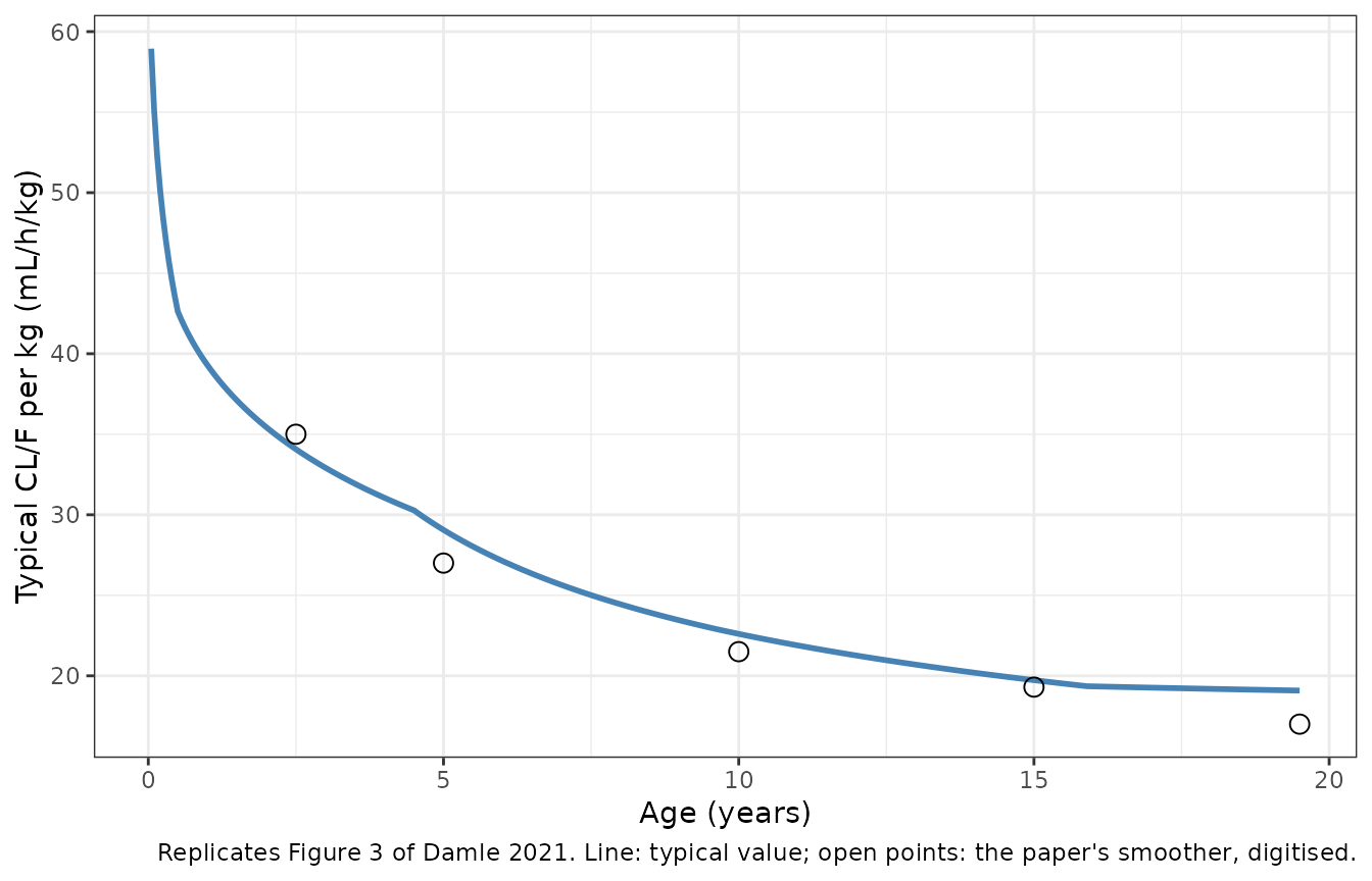

fig3_check <- fig3 |>
  mutate(
    model = typ_cl_per_kg(age),
    pct_diff = 100 * (model - cl_per_kg) / cl_per_kg
  )
knitr::kable(fig3_check, digits = 1)

age	cl_per_kg	model	pct_diff
2.5	35.0	34.1	-2.7
5.0	27.0	29.1	7.6
10.0	21.5	22.6	5.1
15.0	19.3	19.7	2.2
19.5	17.0	19.1	12.3

stopifnot(all(abs(fig3_check$pct_diff) < 15))

At the reference patient (12 years, 43 kg) the typical value is 929 / 43 = 21.6 mL/h/kg.

PKNCA validation

The paper reports no noncompartmental parameters, so the NCA is checked against the closed-form steady-state solution of the one-compartment first-order-absorption model, using each subject’s own CL/F and V/F. Each age group receives the starting dose the paper recommends (150 IU/kg for patients under 2 years, 125 IU/kg for 2 to <8 years and 100 IU/kg from 8 years) every 12 h to steady state.

start_dose <- c(150, 150, 125, 100, 100)
names(start_dose) <- levels(groups$group)
obs_grid <- seq(0, 12, by = 0.1)

ss_prof <- bind_rows(lapply(levels(groups$group), function(g) {
  sub <- filter(cohort, group == g)
  solve_ss(make_events(sub, start_dose[[g]], obs_times = obs_grid)) |>
    mutate(dose_per_kg = start_dose[[g]])
})) |>
  mutate(amt = dose_per_kg * WT)
#> ℹ omega/sigma items treated as zero: 'etalcl'
#> ℹ omega/sigma items treated as zero: 'etalcl'
#> ℹ omega/sigma items treated as zero: 'etalcl'
#> ℹ omega/sigma items treated as zero: 'etalcl'
#> ℹ omega/sigma items treated as zero: 'etalcl'

ss_conc <- ss_prof |>
  filter(!is.na(Cc)) |>
  select(id, group, time, Cc)
ss_dose <- ss_prof |>
  distinct(id, group, amt) |>
  mutate(time = 0)

conc_obj <- PKNCA::PKNCAconc(ss_conc, Cc ~ time | group + id)
dose_obj <- PKNCA::PKNCAdose(ss_dose, amt ~ time | group + id)
intervals <- data.frame(start = 0, end = 12, auclast = TRUE, cmax = TRUE, tmax = TRUE, cmin = TRUE)
nca <- PKNCA::pk.nca(PKNCA::PKNCAdata(conc_obj, dose_obj, intervals = intervals))
nca_res <- as.data.frame(nca$result)

nca_res |>
  select(group, id, PPTESTCD, PPORRES) |>
  pivot_wider(names_from = PPTESTCD, values_from = PPORRES) |>
  group_by(group) |>
  summarise(
    across(c(cmax, tmax, cmin, auclast), ~ signif(median(.x), 3))
  ) |>
  rename(
    `Age group` = group,
    `Cmax,ss (IU/mL)` = cmax,
    `Tmax (h)` = tmax,
    `Cmin,ss (IU/mL)` = cmin,
    `AUC0-12,ss (IU*h/mL)` = auclast
  ) |>
  knitr::kable()

Age group	Cmax,ss (IU/mL)	Tmax (h)	Cmin,ss (IU/mL)	AUC0-12,ss (IU*h/mL)
0 to <8 weeks	0.540	1.6	0.0255	2.72
>=8 weeks to <2 years	0.631	1.8	0.0730	3.84
>=2 to <8 years	0.597	1.9	0.1240	4.25
>=8 to <12 years	0.563	2.0	0.1680	4.39
>=12 to <19 years	0.631	2.1	0.2130	5.09

At steady state AUC(0-12) = Dose / (CL/F), and the 4 h concentration follows the closed-form one-compartment equation. Both sides use the same individual parameters, so the only difference is the trapezoidal and ODE-solver error, and a tight bound applies.

ind <- ss_prof |>
  filter(time == 4) |>
  select(id, group, amt, cl, vc, ka, C4 = Cc)
closed <- nca_res |>
  filter(PPTESTCD == "auclast") |>
  select(id, auc = PPORRES) |>
  inner_join(ind, by = "id") |>
  mutate(
    kel = cl / vc,
    auc_closed = amt / (cl * 1000),
    c4_closed = amt / 1000 * ka / (vc * (ka - kel)) *
      (exp(-kel * 4) / (1 - exp(-kel * 12)) - exp(-ka * 4) / (1 - exp(-ka * 12))),
    auc_pct = 100 * (auc - auc_closed) / auc_closed,
    c4_pct = 100 * (C4 - c4_closed) / c4_closed
  )
closed |>
  group_by(group) |>
  summarise(
    `Max abs AUC diff (%)` = signif(max(abs(auc_pct)), 2),
    `Max abs C4h diff (%)` = signif(max(abs(c4_pct)), 2)
  ) |>
  rename(`Age group` = group) |>
  knitr::kable()

Age group	Max abs AUC diff (%)	Max abs C4h diff (%)
0 to <8 weeks	0.055	4.0e-07
>=8 weeks to <2 years	0.039	2.1e-06
>=2 to <8 years	0.028	6.9e-06
>=8 to <12 years	0.019	1.3e-05
>=12 to <19 years	0.017	2.1e-05

stopifnot(
  nrow(closed) == nrow(cohort),
  all(abs(closed$auc_pct) < 0.5),
  all(abs(closed$c4_pct) < 0.1)
)

Assumptions and deviations

• Additive residual error. Table 2 reports both residual terms as variances (sigma2 P = 0.0519, sigma2 A = 0.016). The text converts the proportional term to its SD (23% CV = sqrt(0.0519)) but quotes the additive term as “0.016 IU/mL”, which is the variance. The model uses SDs for both: propSd = sqrt(0.0519) = 0.228 and addSd = sqrt(0.016) = 0.1265 IU/mL. Both terms enter as independent errors (proportional plus additive).
• Full model, not the reduced model. The model file encodes the full covariate model of Table 2, the only parameter set the paper prints. The paper’s dose simulations used a reduced model with the sex and cancer factors dropped; no separate estimates are reported for it. The simulations above therefore use the full model at its reference levels (female, with cancer), where both factors equal 1. The close agreement with Figure 4 is consistent with the reduced model not having been re-estimated, but the paper does not say.
• Covariate coding. The paper codes SEX = 1 for male and CANCERST = 1 for patients without cancer, and applies each factor when its indicator is 1. The model uses the canonical SEXF (1 = female) and DIS_CANCER_PED (1 = with cancer) columns, with the factors applied as e_sexm_cl^(1 - SEXF) and e_nocancer_cl^(1 - DIS_CANCER_PED). The reference patient is unchanged: a 12-year-old, 43 kg female with cancer.
• Correlated IIV. The paper estimates eta_V/F = theta5 x eta_CL/F, i.e. a correlation of exactly 1. This is encoded as vc_eta_scale * etalcl, because a correlation-1 OMEGA block is singular. The implied V/F variability is 1.73 x 19.2% = 33% CV, matching the text. There is no IIV on ka (the paper removed it because few samples were drawn in the absorption phase).
• Unit conversion. CL/F and V/F are converted from mL to L, and Cc divides by 1000 so anti-Xa activity is in IU/mL.
• Virtual cohort. The paper’s age-weight relationship is not published. The weight-age curve here interpolates the Table 1 group medians, with 20% CV log-normal scatter, 200 subjects per age group (the paper used 1000). The Table 1 weight range for the 2 to <8 years group (11.5-161 kg) includes a value that is implausible for that age and is not used.
• Digitised values. The Figure 4 PTA and overattainment values and the Figure 3 smoother points were read by the maintainers from the published figures and are accurate to roughly +/-0.02 (probability) and +/-1 mL/h/kg.
• Bioavailability. Only subcutaneous dosing was studied, so F is not identifiable. CL/F and V/F are apparent values, and doses go to depot.
• Errata. None found: Crossref lists no correction or update for doi:10.1002/jcph.1716, and the article has no supplementary data beyond its figures (checked 2026-09-27).