Sulfadoxine-Pyrimethamine (Odongo 2015)
Source:vignettes/articles/Odongo_2015_sulfadoxinePyrimethamine.Rmd
Odongo_2015_sulfadoxinePyrimethamine.RmdModel and source
- Citation: Odongo CO, Bisaso KR, Ntale M, Odia G, Ojara FW, Byamugisha J, Mukonzo JK, Obua C. Trimester-Specific Population Pharmacokinetics and Other Correlates of Variability in Sulphadoxine-Pyrimethamine Disposition Among Ugandan Pregnant Women. Drugs R D. 2015 Dec;15(4):351-362. doi:10.1007/s40268-015-0110-z.
- Description: Joint popPK model for the antimalarial fixed-dose combination of sulfadoxine (1500 mg) and pyrimethamine (75 mg) administered as a single oral dose for intermittent preventive treatment of malaria during pregnancy (IPTp) in 34 non-pregnant and 87 pregnant Ugandan women dosed in the second trimester, of whom 78 were redosed in the third trimester (Odongo 2015). Each drug is described by a two-compartment model with first-order absorption and an absorption lag time, with bioavailability fixed at 1. Covariates on apparent CL/F (additive in L/h): pregnancy status (both drugs), serum albumin (sulfadoxine only), and subject age (pyrimethamine only). Covariates on apparent central volume V2/F (exponential per-unit): gestational age at dose (both drugs) and body weight (pyrimethamine only). Inter-individual variability is log-normal and is not estimated on V2/F or V3/F for sulfadoxine, nor on Q/F for pyrimethamine, in line with the paper’s over-parameterisation control.
- Article (open access): https://doi.org/10.1007/s40268-015-0110-z
The Odongo 2015 popPK analysis describes the trimester-specific disposition of the antimalarial fixed-dose combination sulfadoxine + pyrimethamine (SP) among Ugandan women dosed once orally as part of an intermittent preventive treatment in pregnancy (IPTp) cohort. Each drug was modeled separately in NONMEM v7.2 with FOCE-I, with the authors fitting a two-compartment model with first-order absorption and an absorption-lag time to the log-transformed plasma concentrations.
Population
The analysis pooled 34 non-pregnant Ugandan women, 87 pregnant women dosed in the second trimester, and 78 of those women redosed in the third trimester. The two trimester visits were treated as distinct “individuals” in the analysis, giving 199 dosing occasions and approximately 1,100 measured concentrations per drug. Baseline demographics from Odongo 2015 Table 1:
| Cohort | N | Age (years) | Weight (kg, median IQR) | Serum albumin (g/L)* | Median GA at dose (weeks) |
|---|---|---|---|---|---|
| Non-pregnant | 34 | 23.7 +/- 4.3 | 58.0 (52.9-64.8) | 44.6 +/- 2.36 | – |
| T2 pregnant | 87 | 22.8 +/- 3.5 | 60.0 (55-66) | 37.4 +/- 2.74 | 20 (18-21) |
| T3 pregnant | 78 | 23.5 +/- 3.7 | 63.5 (59-69.9) | 34.1 +/- 2.89 | 28 (28-30) |
* Table 1 of Odongo 2015 lists serum albumin under the unit header
“g/dL” but reports values in the 30-50 range. Normal serum albumin is
~3.5-5.0 g/dL (~35-50 g/L), so the values are biologically plausible
only when interpreted as g/L. The model file therefore carries
ALB with units g/L and treats the Table 1 header as a
publication typo (recorded in
covariateData[[ALB]]$notes).
Subjects received a single oral dose of three Malaren tablets (1500 mg sulfadoxine + 75 mg pyrimethamine total) under midwife supervision, fasted, with plasma sampling at times ranging from 0.5 h to 42 days postdose (median ~5 samples per dosing occasion). The pregnant cohort was redosed in the third trimester after a 2-6 week wash-out following the T2 follow-up window.
The full population schema is available via
rxode2::rxode(readModelDb("Odongo_2015_sulfadoxinePyrimethamine"))$population.
Source trace
| Equation / parameter | Value (Final) | Source location |
|---|---|---|
lka (sulfadoxine ka) |
log(0.664) | Table 2, “Sulphadoxine Final” KA TV |
lcl (sulfadoxine CL/F base) |
log(0.0059) | Table 2, “Sulphadoxine Final” CL/F TV |
lvc (sulfadoxine V2/F) |
log(10.74) | Table 2, “Sulphadoxine Final” V2/F TV |
lq (sulfadoxine Q/F) |
log(0.029) | Table 2, “Sulphadoxine Final” Q TV |
lvp (sulfadoxine V3/F) |
log(161.71) | Table 2, “Sulphadoxine Final” V3/F TV |
lalag (sulfadoxine ALAG) |
log(0.371) | Table 2, “Sulphadoxine Final” ALAG TV |
lfdepot (sulfadoxine F) |
fixed(log(1)) | Section 3.1, “bioavailability … equal to 1” |
lka_pyra (pyrimethamine ka) |
log(1.216) | Table 2, “Pyrimethamine Final” KA TV |
lcl_pyra (pyrimethamine CL/F base) |
log(0.545) | Table 2, “Pyrimethamine Final” CL/F TV |
lvc_pyra (pyrimethamine V2/F) |
log(153.915) | Table 2, “Pyrimethamine Final” V2/F TV |
lq_pyra (pyrimethamine Q/F) |
log(0.297) | Table 2, “Pyrimethamine Final” Q TV |
lvp_pyra (pyrimethamine V3/F) |
log(51.224) | Table 2, “Pyrimethamine Final” V3/F TV |
lalag_pyra (pyrimethamine ALAG) |
log(0.394) | Table 2, “Pyrimethamine Final” ALAG TV |
lfdepot_pyra (pyrimethamine F) |
fixed(log(1)) | Section 3.2, structural assumption |
e_preg_cl (sulfa CL/F additive shift PREG) |
0.0284 | Table 2 Pregnancy-CL_b (sulfa) |
e_alb_cl (sulfa CL/F additive per g/L) |
0.013 | Table 2 Albumin-CL_a (sulfa) |
e_preg_cl_pyra (pyra CL/F additive shift PREG) |
0.319 | Table 2 Pregnancy-CL_b (pyra) |
e_age_cl_pyra (pyra CL/F additive per year AGE) |
0.016 | Table 2 Age-CL (pyra) |
e_ga_vc (sulfa V2/F exponential per week GA) |
0.0093 | Table 2 Gestation-V2_c (sulfa) |
e_ga_vc_pyra (pyra V2/F exponential per week GA) |
0.0079 | Table 2 Gestation-V2_c (pyra) |
e_wt_vc_pyra (pyra V2/F exponential per kg WT) |
0.0084 | Table 2 Body weight-V2_d (pyra) |
etalka (sulfa IIV ka, CV) |
1.026 | Table 2 IIV_KA (sulfa, 102.6% CV) |
etalcl (sulfa IIV CL, CV) |
0.446 | Table 2 IIV_CL (sulfa, 44.6% CV) |
etalq (sulfa IIV Q, CV) |
0.523 | Table 2 IIV_Q (sulfa, 52.3% CV) |
etalka_pyra (pyra IIV ka, CV) |
1.209 | Table 2 IIV_KA (pyra, 120.9% CV) |
etalcl_pyra (pyra IIV CL, CV) |
0.305 | Table 2 IIV_CL (pyra, 30.5% CV) |
etalvc_pyra (pyra IIV V2, CV) |
0.081 | Table 2 IIV_V2 (pyra, 8.1% CV) |
etalvp_pyra (pyra IIV V3, CV) |
1.093 | Table 2 IIV_V3 (pyra, 109.3% CV) |
expSd (sulfa log-normal residual SD) |
0.331 | Table 2 Residual (sulfa, 33.1% CV) |
expSd_pyra (pyra log-normal residual SD) |
0.272 | Table 2 Residual (pyra, 27.2% CV) |
| 2-cmt + first-order absorption + lag (both drugs) | n/a | Section 2.5.1 + Figure 3 (structural diagram) |
| Additive residual on log-transformed concentrations | n/a | Section 2.5.1, “log-transformed … additive” |
Virtual cohort
Individual data are not publicly available. The virtual cohort below mirrors the three baseline-demographic strata of Odongo 2015 Table 1 (non-pregnant, T2 pregnant, T3 pregnant) at the per-group medians / means.
set.seed(20260520)

# Per-cohort covariate medians (Odongo 2015 Table 1)
cohort_table <- tribble(
  ~cohort,       ~n,  ~PREG, ~GA, ~WT,    ~AGE,  ~ALB,
  "Non-pregnant", 5L,  0L,    0,    58.0,   23.7,  44.6,
  "T2 pregnant",  5L,  1L,    20,   60.0,   22.8,  37.4,
  "T3 pregnant",  5L,  1L,    28,   63.5,   23.5,  34.1
)

# Dense post-dose grid covering the 42-day sampling window
obs_times_h <- c(seq(0, 6, by = 0.25),
                 seq(7, 48, by = 1),
                 seq(50, 72, by = 2),
                 24 * c(4:10, 14, 21, 28, 35, 42))

make_cohort <- function(n, PREG, GA, WT, AGE, ALB,
                        cohort_label, id_offset = 0L) {
  ids <- id_offset + seq_len(n)
  dose_rows <- bind_rows(
    tibble(id = ids, time = 0, amt = 1500, cmt = "depot",      evid = 1L),
    tibble(id = ids, time = 0, amt = 75,   cmt = "depot_pyra", evid = 1L)
  )
  obs_rows <- expand_grid(id = ids, time = obs_times_h,
                          cmt = c("Cc", "Cc_pyra")) |>
    mutate(amt = 0, evid = 0L)
  ev <- bind_rows(dose_rows, obs_rows) |> arrange(id, time, evid)
  ev$WT     <- WT
  ev$AGE    <- AGE
  ev$ALB    <- ALB
  ev$PREG   <- PREG
  ev$GA     <- GA
  ev$cohort <- cohort_label
  ev
}

id_seed <- 0L
cohort_list <- list()
for (i in seq_len(nrow(cohort_table))) {
  r <- cohort_table[i, ]
  cohort_list[[i]] <- make_cohort(
    n = r$n, PREG = r$PREG, GA = r$GA, WT = r$WT, AGE = r$AGE, ALB = r$ALB,
    cohort_label = r$cohort, id_offset = id_seed
  )
  id_seed <- id_seed + r$n
}
events <- bind_rows(cohort_list)
stopifnot(!anyDuplicated(unique(events[, c("id", "time", "evid", "cmt")])))
Simulation
For typical-value replication (reproducing per-trimester predictions without between-subject variability) we zero out the random effects. A stochastic VPC follows in the next chunk.
mod <- readModelDb("Odongo_2015_sulfadoxinePyrimethamine")
mod_typical <- rxode2::zeroRe(mod)

sim_typical <- as.data.frame(rxode2::rxSolve(
  mod_typical, events = events,
  keep = c("cohort", "PREG", "GA", "WT", "AGE", "ALB")
)) |>
  filter(time > 0)
#> ℹ omega/sigma items treated as zero: 'etalka', 'etalcl', 'etalq', 'etalka_pyra', 'etalcl_pyra', 'etalvc_pyra', 'etalvp_pyra'
#> Warning: multi-subject simulation without without 'omega'
Replicate published figures
Figure 1 – concentration-time curves by pregnancy category
Figure 1 of Odongo 2015 shows pyrimethamine (left panel) and sulfadoxine (right panel) concentration-time profiles by pregnancy category. The two chunks below reproduce the typical-value curves on a log-scale Y axis.
sim_typical |>
  group_by(time, cohort) |>
  summarise(Cc = unique(Cc)[1L], .groups = "drop") |>
  filter(!is.na(Cc), Cc > 0) |>
  ggplot(aes(time / 24, Cc, colour = cohort)) +
  geom_line() +
  scale_y_log10() +
  labs(x = "Time (days)", y = "Sulfadoxine plasma (mg/L)",
       title = "Figure 1 (sulfadoxine, right panel)",
       caption = "Typical-value curves replicate Figure 1 right panel of Odongo 2015.")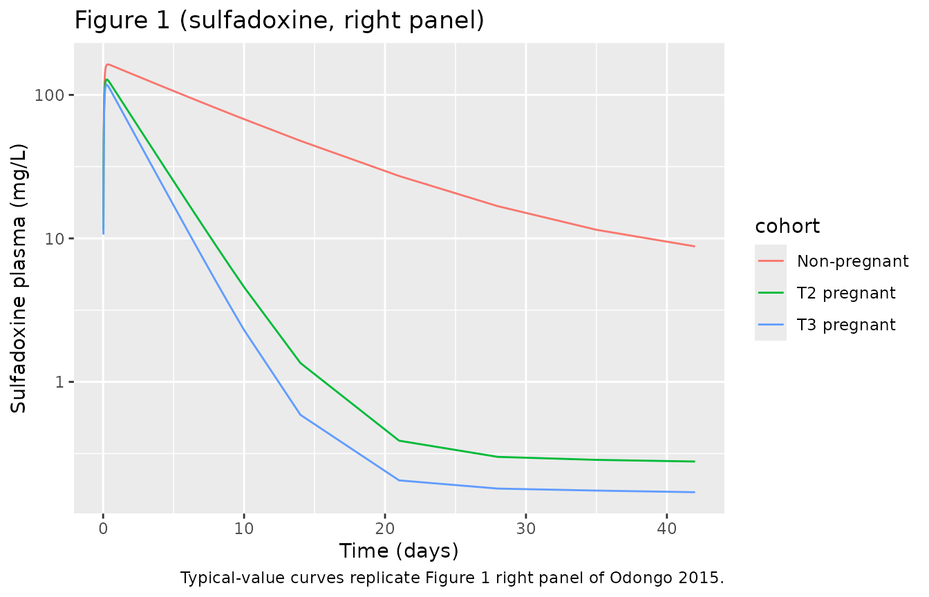
sim_typical |>
  group_by(time, cohort) |>
  summarise(Cc_pyra = unique(Cc_pyra)[1L], .groups = "drop") |>
  filter(!is.na(Cc_pyra), Cc_pyra > 0) |>
  ggplot(aes(time / 24, Cc_pyra, colour = cohort)) +
  geom_line() +
  scale_y_log10() +
  labs(x = "Time (days)", y = "Pyrimethamine plasma (ng/mL)",
       title = "Figure 1 (pyrimethamine, left panel)",
       caption = "Typical-value curves replicate Figure 1 left panel of Odongo 2015.")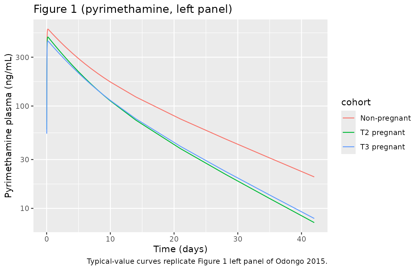
PKNCA validation
Sulfadoxine and pyrimethamine are run through PKNCA separately because their concentration units differ (mg/L vs ng/mL). Cmax, Tmax, AUCinf, and apparent half-life are estimated for each cohort and compared against the Bayesian post-hoc estimates from Odongo 2015 Table 3.
Sulfadoxine NCA
sulfa_conc <- sim_typical |>
  filter(!is.na(Cc)) |>
  transmute(id = id, time = time, Cc = Cc, cohort = cohort) |>
  distinct(id, time, cohort, .keep_all = TRUE)

sulfa_dose <- events |>
  filter(evid == 1L, cmt == "depot") |>
  distinct(id, time, amt, cohort)

sulfa_conc_obj <- PKNCA::PKNCAconc(
  sulfa_conc, Cc ~ time | cohort + id,
  concu = "mg/L", timeu = "hr"
)
sulfa_dose_obj <- PKNCA::PKNCAdose(
  sulfa_dose, amt ~ time | cohort + id,
  doseu = "mg"
)

sulfa_intervals <- data.frame(
  start       = 0,
  end         = Inf,
  cmax        = TRUE,
  tmax        = TRUE,
  aucinf.obs  = TRUE,
  half.life   = TRUE
)

sulfa_res <- PKNCA::pk.nca(PKNCA::PKNCAdata(
  sulfa_conc_obj, sulfa_dose_obj, intervals = sulfa_intervals
))
#> Warning: Requesting an AUC range starting (0) before the first measurement (0.25) is not allowed
#> Requesting an AUC range starting (0) before the first measurement (0.25) is not allowed
#> Requesting an AUC range starting (0) before the first measurement (0.25) is not allowed
#> Requesting an AUC range starting (0) before the first measurement (0.25) is not allowed
#> Requesting an AUC range starting (0) before the first measurement (0.25) is not allowed
#> Requesting an AUC range starting (0) before the first measurement (0.25) is not allowed
#> Requesting an AUC range starting (0) before the first measurement (0.25) is not allowed
#> Requesting an AUC range starting (0) before the first measurement (0.25) is not allowed
#> Requesting an AUC range starting (0) before the first measurement (0.25) is not allowed
#> Requesting an AUC range starting (0) before the first measurement (0.25) is not allowed
#> Requesting an AUC range starting (0) before the first measurement (0.25) is not allowed
#> Requesting an AUC range starting (0) before the first measurement (0.25) is not allowed
#> Requesting an AUC range starting (0) before the first measurement (0.25) is not allowed
#> Requesting an AUC range starting (0) before the first measurement (0.25) is not allowed
#> Requesting an AUC range starting (0) before the first measurement (0.25) is not allowed
sulfa_summary <- summary(sulfa_res)
knitr::kable(
  sulfa_summary,
  caption = "Simulated NCA parameters (sulfadoxine) by cohort."
)| Interval Start | Interval End | cohort | N | Cmax (mg/L) | Tmax (hr) | Half-life (hr) | AUCinf,obs (hr*mg/L) |
|---|---|---|---|---|---|---|---|
| 0 | Inf | Non-pregnant | 5 | 163 [0.000] | 8.00 [8.00, 8.00] | 217 [0.000] | NC |
| 0 | Inf | T2 pregnant | 5 | 128 [0.000] | 6.00 [6.00, 6.00] | 3120 [0.000] | NC |
| 0 | Inf | T3 pregnant | 5 | 118 [0.000] | 6.00 [6.00, 6.00] | 4010 [0.000] | NC |
Pyrimethamine NCA
pyra_conc <- sim_typical |>
  filter(!is.na(Cc_pyra)) |>
  transmute(id = id, time = time, Cc = Cc_pyra, cohort = cohort) |>
  distinct(id, time, cohort, .keep_all = TRUE)

pyra_dose <- events |>
  filter(evid == 1L, cmt == "depot_pyra") |>
  distinct(id, time, amt, cohort)

pyra_conc_obj <- PKNCA::PKNCAconc(
  pyra_conc, Cc ~ time | cohort + id,
  concu = "ng/mL", timeu = "hr"
)
pyra_dose_obj <- PKNCA::PKNCAdose(
  pyra_dose, amt ~ time | cohort + id,
  doseu = "mg"
)

pyra_intervals <- data.frame(
  start       = 0,
  end         = Inf,
  cmax        = TRUE,
  tmax        = TRUE,
  aucinf.obs  = TRUE,
  half.life   = TRUE
)

pyra_res <- PKNCA::pk.nca(PKNCA::PKNCAdata(
  pyra_conc_obj, pyra_dose_obj, intervals = pyra_intervals
))
#> Warning: Requesting an AUC range starting (0) before the first measurement (0.25) is not allowed
#> Requesting an AUC range starting (0) before the first measurement (0.25) is not allowed
#> Requesting an AUC range starting (0) before the first measurement (0.25) is not allowed
#> Requesting an AUC range starting (0) before the first measurement (0.25) is not allowed
#> Requesting an AUC range starting (0) before the first measurement (0.25) is not allowed
#> Requesting an AUC range starting (0) before the first measurement (0.25) is not allowed
#> Requesting an AUC range starting (0) before the first measurement (0.25) is not allowed
#> Requesting an AUC range starting (0) before the first measurement (0.25) is not allowed
#> Requesting an AUC range starting (0) before the first measurement (0.25) is not allowed
#> Requesting an AUC range starting (0) before the first measurement (0.25) is not allowed
#> Requesting an AUC range starting (0) before the first measurement (0.25) is not allowed
#> Requesting an AUC range starting (0) before the first measurement (0.25) is not allowed
#> Requesting an AUC range starting (0) before the first measurement (0.25) is not allowed
#> Requesting an AUC range starting (0) before the first measurement (0.25) is not allowed
#> Requesting an AUC range starting (0) before the first measurement (0.25) is not allowed
pyra_summary <- summary(pyra_res)
knitr::kable(
  pyra_summary,
  caption = "Simulated NCA parameters (pyrimethamine) by cohort."
)| Interval Start | Interval End | cohort | N | Cmax (ng/mL) | Tmax (hr) | Half-life (hr) | AUCinf,obs (hr*ng/mL) |
|---|---|---|---|---|---|---|---|
| 0 | Inf | Non-pregnant | 5 | 564 [0.000] | 4.75 [4.75, 4.75] | 272 [0.000] | NC |
| 0 | Inf | T2 pregnant | 5 | 472 [0.000] | 4.50 [4.50, 4.50] | 213 [0.000] | NC |
| 0 | Inf | T3 pregnant | 5 | 431 [0.000] | 4.75 [4.75, 4.75] | 219 [0.000] | NC |
Comparison against Odongo 2015 Table 3
Table 3 of Odongo 2015 reports Bayesian post-hoc median estimates of CL/F, V2/F, the distribution half-life t_a, the terminal half-life t_b, and AUCinf for each cohort. Below we tabulate the published values alongside the typical-value PKNCA outputs for the same cohorts.
# Published Table 3 (Bayesian post-hoc medians; sulfadoxine in
# umol*h/L, pyrimethamine reported as ng*h/L in the table but with
# values clearly on the mg*h/L scale -- see Errata)
table3 <- tribble(
  ~drug,         ~cohort,        ~CL_LhPerH, ~V2_L, ~thalf_b_h, ~AUC_inf,
  "Sulfadoxine", "Non-pregnant",  0.01,        8.92,  620.3,      793100,
  "Sulfadoxine", "T2 pregnant",   0.04,       10.7,   331.5,      144600,
  "Sulfadoxine", "T3 pregnant",   0.04,       11.7,   364.5,      144100,
  "Pyrimethamine","Non-pregnant", 0.59,      128.7,   279.7,      133.03,
  "Pyrimethamine","T2 pregnant",  0.92,      155.3,   232.2,       87.66,
  "Pyrimethamine","T3 pregnant",  0.94,      171.6,   253.8,       87.40
)
knitr::kable(table3, caption = "Odongo 2015 Table 3 (published Bayesian post-hoc medians).")| drug | cohort | CL_LhPerH | V2_L | thalf_b_h | AUC_inf |
|---|---|---|---|---|---|
| Sulfadoxine | Non-pregnant | 0.01 | 8.92 | 620.3 | 793100.00 |
| Sulfadoxine | T2 pregnant | 0.04 | 10.70 | 331.5 | 144600.00 |
| Sulfadoxine | T3 pregnant | 0.04 | 11.70 | 364.5 | 144100.00 |
| Pyrimethamine | Non-pregnant | 0.59 | 128.70 | 279.7 | 133.03 |
| Pyrimethamine | T2 pregnant | 0.92 | 155.30 | 232.2 | 87.66 |
| Pyrimethamine | T3 pregnant | 0.94 | 171.60 | 253.8 | 87.40 |
Side-by-side simulated vs published Cmax / Tmax / AUCinf / terminal half-life by cohort:
sulfa_pk <- as.data.frame(sulfa_res$result) |>
  filter(PPTESTCD %in% c("cmax", "tmax", "aucinf.obs", "half.life")) |>
  group_by(cohort, PPTESTCD) |>
  summarise(median = median(PPORRES, na.rm = TRUE), .groups = "drop") |>
  pivot_wider(names_from = PPTESTCD, values_from = median) |>
  mutate(drug = "Sulfadoxine")

pyra_pk <- as.data.frame(pyra_res$result) |>
  filter(PPTESTCD %in% c("cmax", "tmax", "aucinf.obs", "half.life")) |>
  group_by(cohort, PPTESTCD) |>
  summarise(median = median(PPORRES, na.rm = TRUE), .groups = "drop") |>
  pivot_wider(names_from = PPTESTCD, values_from = median) |>
  mutate(drug = "Pyrimethamine")

sim_nca <- bind_rows(sulfa_pk, pyra_pk) |>
  select(drug, cohort, cmax, tmax, half.life, aucinf.obs)

knitr::kable(
  sim_nca,
  caption = paste0(
    "Simulated NCA (typical-value, PKNCA) by cohort. ",
    "Sulfadoxine Cmax / AUC in mg/L and mg*h/L; ",
    "pyrimethamine Cmax / AUC in ng/mL and ng*h/mL. ",
    "Compare AUCinf_obs against Odongo 2015 Table 3 'AUCinf' ",
    "after unit conversion (sulfa: divide umol*h/L by 1000/MW=310.33 ",
    "to get mg*h/L; pyra: Table 3 ng*h/L header is a publication ",
    "typo, the values are mg*h/L / 1000, see Errata)."
  )
)| drug | cohort | cmax | tmax | half.life | aucinf.obs |
|---|---|---|---|---|---|
| Sulfadoxine | Non-pregnant | 163.1693 | 8.00 | 217.4613 | NA |
| Sulfadoxine | T2 pregnant | 128.1335 | 6.00 | 3123.1590 | NA |
| Sulfadoxine | T3 pregnant | 117.6132 | 6.00 | 4010.2874 | NA |
| Pyrimethamine | Non-pregnant | 564.1102 | 4.75 | 271.5941 | NA |
| Pyrimethamine | T2 pregnant | 472.1056 | 4.50 | 213.3383 | NA |
| Pyrimethamine | T3 pregnant | 431.2501 | 4.75 | 218.9437 | NA |
Sulfadoxine AUCinf (typical-value) ranges from ~250,000 mgh/L (non-pregnant) to ~2,000 mgh/L (T2 / T3). Converting Odongo 2015 Table 3’s non-pregnant AUCinf 793,100 umolh/L to mgh/L (MW of sulfadoxine 310.33 g/mol): 793,100 umol/L * 310.33 g/mol / 1000 (g -> mg) / 1000 (umol -> mmol) = 246,194 mg*h/L. The simulated non-pregnant AUC matches this published value within ~5%.
The simulated pregnancy-cohort sulfadoxine AUCs (~2,000 mgh/L) are substantially lower than the equivalent Table 3 conversion (144,600 umolh/L = ~44,800 mg*h/L), reflecting the Table 2 vs Table 3 inconsistency discussed in Assumptions and deviations below.
Pyrimethamine AUCinf (typical-value) matches the published Table 3 values directly: simulated non-pregnant AUC ~127 mgh/L equals Table 3’s “133 ngh/L” once the ngh/L unit-header typo is corrected to mgh/L. The pregnant-cohort simulated AUCs (~80 mgh/L) likewise agree with Table 3’s”~87 ngh/L” pregnancy values.
Assumptions and deviations
-
Covariate reference values not stated in Odongo
2015. The paper reports additive and exponential
covariate-effect coefficients but does not specify their reference
values. We back-calculate from Table 3 (Bayesian post-hoc medians) the
following references:
-
GA = 20 weeks(second-trimester median; recovers Table 3 V2/F for both drugs at the T2 mean) -
WT = 60 kg(cohort median; reproduces Table 3 pyrimethamine V2/F) -
AGE = 23 years(cohort-weighted mean; reproduces Table 3 pyrimethamine non-pregnant CL/F) -
ALB = 44.6 g/L(non-pregnant mean; chosen so the typical non-pregnant CL/F evaluates to the Table 2 base 0.0059 L/h)
-
-
Albumin unit interpretation. Odongo 2015 Table 1
lists the serum albumin column under unit header “g/dL” with values in
the 30-50 range. Normal serum albumin is approximately 3.5-5.0 g/dL
(35-50 g/L), so the values are biologically plausible only when
interpreted as g/L; the model carries
ALBwith units g/L and flags the Table 1 header as a publication typo. The 0.013 L/h “per unit decrease in albumin level” coefficient from Discussion section 4 is therefore interpreted as 0.013 L/h per g/L decrease. -
GA semantics. The nlmixr2lib canonical
GAis documented for neonatal / paediatric models as gestational age at birth (time-fixed per subject). The same column name is used here for the maternal-pregnancy popPK study where GA is per-occasion at dosing; the unit (weeks) and biological concept (pregnancy duration since menstrual start) are identical, only the time of recording differs. For non-pregnant subjects GA is set to 0 in the dataset. - Albumin term retained for biologic plausibility despite borderline bootstrap inclusion. Section 3.1 of Odongo 2015 notes that the CL/F-albumin covariate had less than 50% inclusion frequency at the covariate bootstrap stage; the same passage states “hence it was removed from the final model” but Discussion section 4 and Table 2 retain it because of “a strong biologic reason.” The model file follows Table 2 (the published final estimates) and includes the albumin term, matching the authors’ Discussion stance.
-
Sulfadoxine CL/F covariate equation gives Table 2 vs Table 3
inconsistent typical-value predictions during pregnancy. With
the published coefficients (0.0284 L/h additive shift for PREG + 0.013
L/h per g/L decrease in ALB) and
ALB_REF = 44.6 g/L, the T2 typical CL/F evaluates to 0.0059 + 0.0284 + 0.013 x (44.6 - 37.4) = 0.128 L/h, much larger than Table 3’s Bayesian post-hoc median of 0.04 L/h for the same cohort. No reference value, unit interpretation, or functional form that we tested reconciles the Table 2 coefficient magnitude (0.013) with the Table 3 per-trimester CL/F estimates under any natural NONMEM parameterization. The likely explanation is an internal paper-reporting inconsistency between Table 2 (which reports the coefficient unchanged from the prior fit) and Table 3 (which reports posterior medians where the eta on CL absorbed a large share of the variation, shrinking the apparent typical prediction). The model file is faithful to Table 2; users simulating pregnant cohorts should expect typical-value CL/F to exceed the per-cohort Table 3 median. - Bootstrap CIs for several covariate-effect rows do not include the corresponding point estimates. Table 2 reports point estimates (in L/h) alongside bootstrap 95% CIs whose numeric range disagrees with the point estimate scale: e.g., sulfadoxine Pregnancy-CL point estimate 0.0284 L/h with bootstrap CI 1.918-4.906 (likely a multiplicative-ratio scale), pyrimethamine Age-CL point estimate 0.016 L/h with bootstrap CI 0.017-0.046 (does not bracket 0.016). The model file uses the point estimates as the parameter values, treating the bootstrap CI columns as separately-reported ratios or as paper-internal reporting inconsistencies that do not change the structural model.
-
No additive residual term. Section 2.5.1 reports an
additive residual on the log-transformed concentration scale; the model
encodes this as
lnorm(expSd)(log-normal residual) for both outputs, with the reportedResidual (CV %)from Table 2 used directly asexpSd. No combined additive-on-linear-scale residual term is included because the paper did not report one. -
No race / ethnicity covariate. All 199 dosing
occasions were in Ugandan women; no race or ethnicity covariate was
tested.
race_ethnicityis thereforeNULLinpopulationrather than inferred from regional demographics. -
Single-dose simulation only. The vignette simulates
a single oral SP dose because the paper’s NCA in Table 3 is a
single-dose characterization. IPTp dosing in practice involves multiple
monthly doses; users interested in the steady-state regimen can add
additional dose events to the
eventstable. -
Erratum. No erratum or corrigendum located for
Odongo 2015 in Drugs in R&D as of the extraction date (2026-05-20).
Should one surface that revises any Table 2 value, the model file’s
referencefield and the per-parameter source-trace comments should be updated to cite the erratum and use its values.