Dupilumab (Kovalenko 2020)
Source:vignettes/articles/Kovalenko_2020_dupilumab.Rmd
Kovalenko_2020_dupilumab.RmdModel and source
- Citation: Kovalenko P, Davis JD, Li M, et al. Base and Covariate Population Pharmacokinetic Analyses of Dupilumab Using Phase 3 Data. Clinical Pharmacology in Drug Development. 2020;9(6):756-767. doi:10.1002/cpdd.780
- Article: Clin Pharmacol Drug Dev. 2020;9(6):756-767 (open access via PMC7496533)
Kovalenko 2020 reports four sequential popPK models for dupilumab built using a stepwise approach:
-
Model 1 – rich Phase 1/2 data with all structural
parameters estimated. Available as
readModelDb("Kovalenko_2020_dupilumab"). - Model 2 – 12 Phase 1/2 studies, used to test population (healthy vs AD) and assay-version covariates; neither was retained. Not packaged separately.
-
Model 3 – primary BASE model fit to Phase 3
atopic-dermatitis data with most structural parameters FIXED to Model
1/2 values; only body weight enters as a covariate of central volume.
Available as
readModelDb("Kovalenko_2020_dupilumab_base"). -
Model 4 – primary COVARIATE model on the same Phase
3 data, adding albumin to Vc and BMI / EASI / race (White) to the linear
elimination rate ke. Available as
readModelDb("Kovalenko_2020_dupilumab_covariate").
This vignette walks all three packaged models (1, 3, 4) and validates simulated typical-subject steady-state exposure against PKNCA-derived metrics.
Population
Kovalenko 2020 pooled 16 clinical studies (N = 2115 participants; 202 healthy volunteers and 1913 patients with moderate-to-severe atopic dermatitis (AD)). Of these, 2041 participants on active treatment contributed 18,243 of 20,809 samples to the population PK analysis. Source studies include the Phase 3 AD trials R668-AD-1334 (LIBERTY AD SOLO 1), R668-AD-1416 (LIBERTY AD SOLO 2), and R668-AD-1224 (LIBERTY AD CHRONOS). The Phase 1 studies R668-AS-0907, TDU12265, PKM14161, and R668-AD-1117 were used to fit Model 1; the Phase 3 trials alone were used for Models 3 and 4. The paper’s main text does not tabulate detailed baseline demographics for the pooled cohort; per-study geographic locations and dosing regimens appear in Supplementary Table S1.
The approved adult AD maintenance regimen is 600 mg SC loading dose on day 0 followed by 300 mg SC every 2 weeks (Q2W); the Kovalenko 2016 precursor publication used 75 kg as the reference body weight for the allometric effect on central volume, and the 2020 paper reuses the same equation without re-stating the reference weight.
The same information is available programmatically via
readModelDb("Kovalenko_2020_dupilumab")$population,
readModelDb("Kovalenko_2020_dupilumab_base")$population,
and
readModelDb("Kovalenko_2020_dupilumab_covariate")$population.
Source trace
Every structural parameter, covariate effect, IIV element, and
residual-error term in the three packaged models is taken from Kovalenko
2020 Table 1 (Model 1 column), Supplementary Table S2 (Model 1 IIV /
residual error), and Supplementary Table S3 (Models 3 and 4). The
per-parameter origin is recorded as an in-file comment next to each
ini() entry in the three model files; the cross-walks below
collect them in one place for review.
Model 1 – rich-data exploratory fit
(Kovalenko_2020_dupilumab)
| Equation / parameter | Value | Source location |
|---|---|---|
lvc (Vc, central volume) |
log(2.48) L |
Table 1, Model 1 |
lkel (ke, linear elimination rate) |
log(0.0534) 1/day |
Table 1, Model 1 |
lkcp (kcp) |
log(0.213) 1/day |
Table 1, Model 1 |
Mpc (kcp/kpc) |
0.686 |
Table 1, Model 1 (kpc derived: 0.213 / 0.686 = 0.310 1/day) |
lka (ka, absorption rate) |
log(0.256) 1/day |
Table 1, Model 1 |
lmtt (MTT) |
log(0.105) day |
Table 1, Model 1 |
lvmax (Vmax) |
log(1.07) mg/L/day |
Table 1, Model 1 |
Km |
fixed(0.01) mg/L |
Table 1, Model 1 (fixed, carried over from Kovalenko 2016) |
lfdepot (F) |
log(0.643) |
Table 1, Model 1 |
e_wt_vc (WT exponent on Vc) |
0.711 |
Table 1, Model 1 (“Vc ~ weight”) |
var(etalvc) |
0.192^2 = 0.036864 |
Supp. Table S2: omega_Vc (SD) = 0.192 |
var(etalkel) |
0.285^2 = 0.081225 |
Supp. Table S2: omega_ke (SD) = 0.285 |
var(etalka) |
0.474^2 = 0.224676 |
Supp. Table S2: omega_ka (SD) = 0.474 |
var(etalvmax) |
0.236^2 = 0.055696 |
Supp. Table S2: omega_Vm (SD) = 0.236 |
var(etalmtt) |
0.525^2 = 0.275625 |
Supp. Table S2: omega_MTT (SD) = 0.525, applied on
log(MTT) here |
propSd (proportional sigma) |
0.15 |
Supp. Table S2 |
addSd (additive sigma) |
fixed(0.03) mg/L |
Supp. Table S2 (fixed, carried over from Kovalenko 2016) |
| Structure | 2-cmt + 3 transit + parallel linear/MM elimination | p. 758 Methods, Figure 1 |
Model 3 – primary base model on Phase 3 data
(Kovalenko_2020_dupilumab_base)
| Equation / parameter | Value | Source location |
|---|---|---|
lvc (Vc) |
log(2.76) L |
Supp. Table S3 Model 3 / Table 1 |
lkel (ke) |
log(0.0448) 1/day |
Supp. Table S3 Model 3 / Table 1 |
lkcp |
fixed(log(0.211)) 1/day |
Supp. Table S3 Model 3 (fixed) |
lkpc |
fixed(log(0.310)) 1/day |
Supp. Table S3 Model 3 (fixed) |
lka |
fixed(log(0.306)) 1/day |
Supp. Table S3 Model 3 (fixed) |
lmtt |
fixed(log(0.105)) day |
Supp. Table S3 Model 3 (fixed) |
lvmax |
fixed(log(1.07)) mg/L/day |
Supp. Table S3 Model 3 (fixed) |
Km |
fixed(0.01) mg/L |
Supp. Table S3 Model 3 (fixed) |
lfdepot |
fixed(log(0.642)) |
Supp. Table S3 Model 3 (fixed) |
e_wt_vc (WT exponent on Vc) |
0.919 |
Supp. Table S3 Model 3 (“Vc ~ weight”) |
var(etalvc) |
0.216^2 = 0.046656 |
Supp. Table S3: sigma(ln Vc) = 0.216 |
var(etalkel) |
0.301^2 = 0.090601 |
Supp. Table S3: sigma(ln ke) = 0.301 |
cov(etalvc, etalkel) |
-0.373 * 0.216 * 0.301 = -0.024254 |
Supp. Table S3: Corr(ln ke, ln Vc) = -0.373 |
propSd |
0.124 |
Supp. Table S3: sigma_prop (CV%) = 12.4 |
addSd |
6.17 mg/L |
Supp. Table S3: sigma_add = 6.17 mg/L |
Model 4 – primary covariate model on Phase 3 data
(Kovalenko_2020_dupilumab_covariate)
| Equation / parameter | Value | Source location |
|---|---|---|
lvc (Vc) |
log(2.74) L |
Supp. Table S3 Model 4 / Table 1 |
lkel (ke) |
log(0.0477) 1/day |
Supp. Table S3 Model 4 / Table 1 |
| Fixed parameters (kcp, kpc, ka, MTT, Vm, Km, F) | same as Model 3 | Supp. Table S3 Model 4 |
e_wt_vc (WT exponent on Vc) |
0.817 |
Supp. Table S3 Model 4 / Table 3 |
e_alb_vc (ALB exponent on Vc) |
-0.653 |
Supp. Table S3 Model 4 / Table 3 |
e_bmi_kel (BMI exponent on ke) |
0.368 |
Supp. Table S3 Model 4 / Table 3 |
e_score_easi_kel (EASI exponent on ke) |
0.143 |
Supp. Table S3 Model 4 / Table 3 |
e_race_white_kel (race White on ke) |
-0.123 |
Supp. Table S3 Model 4 / Table 3 |
var(etalvc) |
0.206^2 = 0.042436 |
Supp. Table S3: sigma(ln Vc) = 0.206 |
var(etalkel) |
0.293^2 = 0.085849 |
Supp. Table S3: sigma(ln ke) = 0.293 |
cov(etalvc, etalkel) |
-0.450 * 0.206 * 0.293 = -0.0271611 |
Supp. Table S3: Corr(ln ke, ln Vc) = -0.450 |
propSd |
0.125 |
Supp. Table S3: sigma_prop (CV%) = 12.5 |
addSd |
6.06 mg/L |
Supp. Table S3: sigma_add = 6.06 mg/L |
The paper’s Methods explicitly define omega as “omega (omega,
standard deviation [SD] of between-subject variability)” and sigma
as “sigma (sigma, SD of measurement error)”. nlmixr2’s
etalxxx ~ value syntax stores the variance
(omega^2), so the SDs from Table S2 / S3 are squared in
ini(). For Models 3 and 4 the IIV is a correlated block on
(ln Vc, ln ke); the covariance is computed from the published
correlation inline in each model file’s ini().
Parameterization notes
All three models share the same structural form: a 2-compartment PK
with parallel linear (kel * central) and Michaelis-Menten
(vmax * central / (Km + central/vc)) elimination, fed by a
3-transit- compartment SC absorption chain (ktr = 4 / MTT).
Intercompartmental transport is parameterized as direct rate constants
kcp and kpc (equivalently k12,
k21) rather than as Q / Vp. IV doses bypass the depot via
the event record; the SC bioavailability fdepot applies on
the depot compartment only.
Virtual cohort
Detailed observed demographics for the pooled cohort are not publicly reproduced in the paper’s main text. The virtual cohort below targets the labelled adult AD population using covariate distributions consistent with the LIBERTY AD SOLO 1/2 (Simpson 2016 doi:10.1056/NEJMoa1610020 Table 1) and CHRONOS (Blauvelt 2017 doi:10.1016/S0140-6736(17)31191-1 Table 1) Phase 3 publications. All five covariates needed by Model 4 are drawn for every subject so the same event table can be reused for Models 1, 3, and 4.
set.seed(20260621)
n_subj <- 200

draw_trunc_norm <- function(n, mean, sd, lo, hi) {
  pmin(pmax(rnorm(n, mean = mean, sd = sd), lo), hi)
}

cohort <- tibble::tibble(
  id         = seq_len(n_subj),
  WT         = draw_trunc_norm(n_subj, mean = 75, sd = 18, lo = 40, hi = 165),
  ALB        = draw_trunc_norm(n_subj, mean = 44, sd =  4, lo = 30, hi =  55),
  BMI        = draw_trunc_norm(n_subj, mean = 27, sd =  5, lo = 18, hi =  45),
  SCORE_EASI = draw_trunc_norm(n_subj, mean = 32, sd = 12, lo = 16, hi =  72),
  RACE_WHITE = as.integer(runif(n_subj) < 0.67)
)

# Labelled AD regimen: 600 mg SC loading dose on day 0, 300 mg SC Q2W for
# 12 additional doses -> study window 0-182 days.  By dose 10+ the profile
# is close to steady state (typical half-life ~2-3 weeks).
load_dose  <- 600
maint_dose <- 300
tau        <- 14
n_maint    <- 12
dose_days  <- c(0, seq(tau, tau * n_maint, by = tau))
amt_vec    <- c(load_dose, rep(maint_dose, n_maint))

ev_dose <- cohort |>
  tidyr::crossing(time = dose_days) |>
  dplyr::arrange(id, time) |>
  dplyr::group_by(id) |>
  dplyr::mutate(amt = amt_vec, cmt = "depot", evid = 1L) |>
  dplyr::ungroup()

obs_days <- sort(unique(c(
  seq(0, tau * (n_maint + 1), by = 1),
  dose_days + 0.25,
  dose_days + 1,
  dose_days + 3
)))

# Observation rows reference the ODE state "central" (not the observable
# "Cc") to avoid the rxode2 slot-renumbering bug; the observable Cc is
# returned automatically alongside the central amount.
ev_obs <- cohort |>
  tidyr::crossing(time = obs_days) |>
  dplyr::mutate(amt = 0, cmt = "central", evid = 0L)

events <- dplyr::bind_rows(ev_dose, ev_obs) |>
  dplyr::arrange(id, time, dplyr::desc(evid)) |>
  dplyr::select(id, time, amt, cmt, evid, WT, ALB, BMI, SCORE_EASI, RACE_WHITE)
Model 1 – rich-data exploratory fit
mod_m1 <- rxode2::rxode2(readModelDb("Kovalenko_2020_dupilumab"))
#> ℹ parameter labels from comments will be replaced by 'label()'
conc_unit <- mod_m1$units[["concentration"]]
sim_m1 <- rxode2::rxSolve(mod_m1, events = events,
                          keep = c("WT", "ALB", "BMI", "SCORE_EASI", "RACE_WHITE"))
Figure replication – Cc vs time (Model 1)
Reproduces the labelled adult AD regimen (600 mg SC loading + 300 mg SC Q2W) as 5th / 50th / 95th percentile bands across the virtual cohort, spanning ~13 dosing cycles (cf. Kovalenko 2020 Figure 5).
vpc_m1 <- sim_m1 |>
  dplyr::filter(!is.na(Cc), time > 0) |>
  dplyr::group_by(time) |>
  dplyr::summarise(
    Q05 = quantile(Cc, 0.05, na.rm = TRUE),
    Q50 = quantile(Cc, 0.50, na.rm = TRUE),
    Q95 = quantile(Cc, 0.95, na.rm = TRUE),
    .groups = "drop"
  )

ggplot(vpc_m1, aes(time, Q50)) +
  geom_ribbon(aes(ymin = Q05, ymax = Q95), alpha = 0.2, fill = "#4682b4") +
  geom_line(colour = "#4682b4", linewidth = 0.8) +
  geom_vline(xintercept = dose_days, linetype = "dotted", colour = "grey70") +
  scale_y_continuous(limits = c(0, NA)) +
  labs(
    x = "Time (days)",
    y = paste0("Dupilumab Cc (", conc_unit, ")"),
    title = "Model 1 (rich-data fit): simulated 5-50-95 percentile profile",
    caption = "600 mg SC load then 300 mg SC Q2W; virtual AD cohort N = 200."
  ) +
  theme_minimal()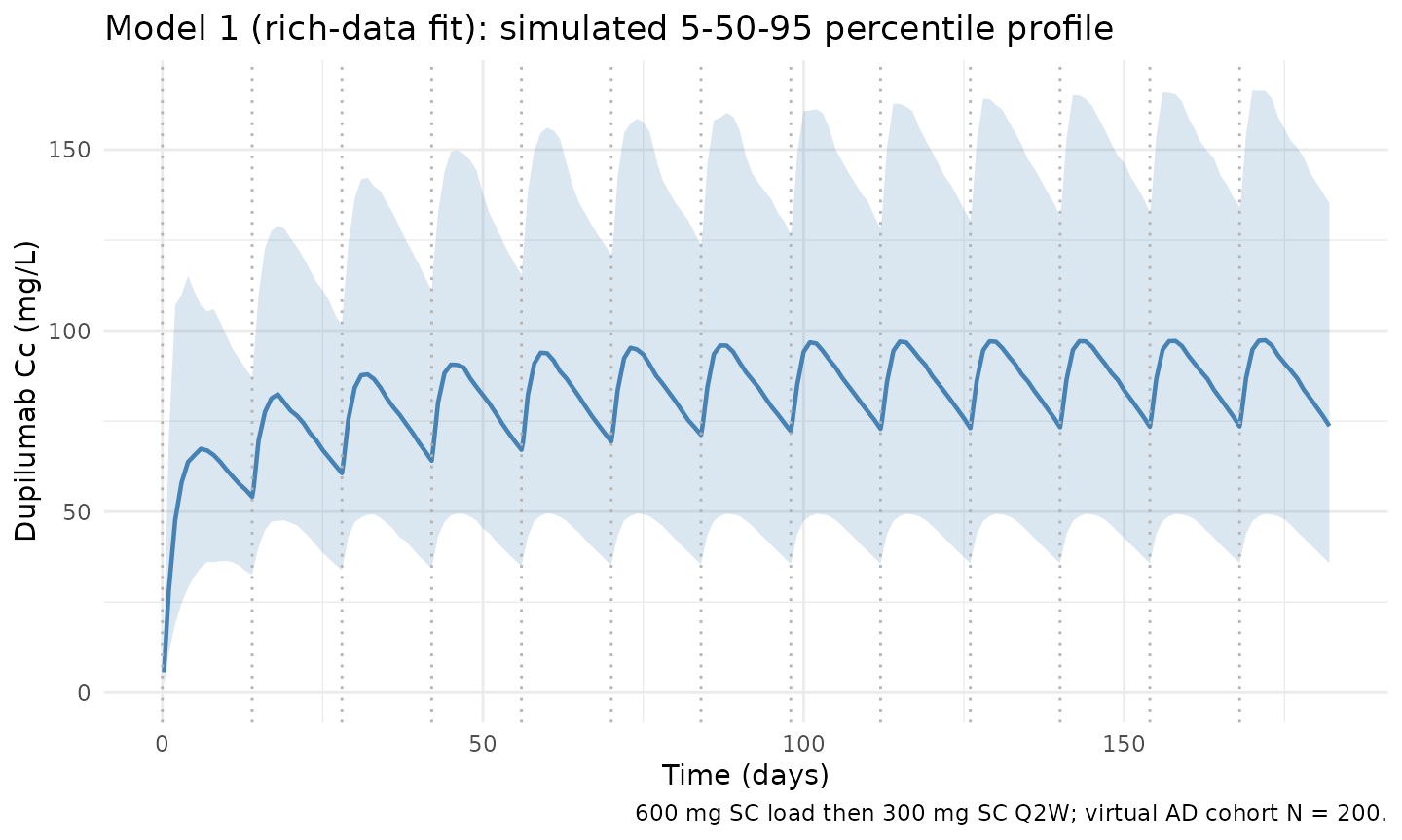
Model 3 – primary base model on Phase 3 data
mod_m3 <- rxode2::rxode2(readModelDb("Kovalenko_2020_dupilumab_base"))
sim_m3 <- rxode2::rxSolve(mod_m3, events = events,
                          keep = c("WT", "ALB", "BMI", "SCORE_EASI", "RACE_WHITE"))
VPC profile (Model 3)
vpc_m3 <- sim_m3 |>
  dplyr::filter(!is.na(Cc), time > 0) |>
  dplyr::group_by(time) |>
  dplyr::summarise(
    Q05 = quantile(Cc, 0.05, na.rm = TRUE),
    Q50 = quantile(Cc, 0.50, na.rm = TRUE),
    Q95 = quantile(Cc, 0.95, na.rm = TRUE),
    .groups = "drop"
  )

ggplot(vpc_m3, aes(time, Q50)) +
  geom_ribbon(aes(ymin = Q05, ymax = Q95), alpha = 0.2, fill = "#4682b4") +
  geom_line(colour = "#4682b4", linewidth = 0.8) +
  geom_vline(xintercept = dose_days, linetype = "dotted", colour = "grey70") +
  scale_y_continuous(limits = c(0, NA)) +
  labs(
    x = "Time (days)",
    y = paste0("Dupilumab Cc (", conc_unit, ")"),
    title = "Model 3 (primary base, Phase 3): simulated 5-50-95 percentile profile",
    caption = "600 mg SC load then 300 mg SC Q2W; virtual AD cohort N = 200."
  ) +
  theme_minimal()
Model 4 – primary covariate model on Phase 3 data
mod_m4 <- rxode2::rxode2(readModelDb("Kovalenko_2020_dupilumab_covariate"))
sim_m4 <- rxode2::rxSolve(mod_m4, events = events,
                          keep = c("WT", "ALB", "BMI", "SCORE_EASI", "RACE_WHITE"))
VPC profile (Model 4)
vpc_m4 <- sim_m4 |>
  dplyr::filter(!is.na(Cc), time > 0) |>
  dplyr::group_by(time) |>
  dplyr::summarise(
    Q05 = quantile(Cc, 0.05, na.rm = TRUE),
    Q50 = quantile(Cc, 0.50, na.rm = TRUE),
    Q95 = quantile(Cc, 0.95, na.rm = TRUE),
    .groups = "drop"
  )

ggplot(vpc_m4, aes(time, Q50)) +
  geom_ribbon(aes(ymin = Q05, ymax = Q95), alpha = 0.2, fill = "#b4464b") +
  geom_line(colour = "#b4464b", linewidth = 0.8) +
  geom_vline(xintercept = dose_days, linetype = "dotted", colour = "grey70") +
  scale_y_continuous(limits = c(0, NA)) +
  labs(
    x = "Time (days)",
    y = paste0("Dupilumab Cc (", conc_unit, ")"),
    title = "Model 4 (primary covariate, Phase 3): simulated 5-50-95 percentile profile",
    caption = "600 mg SC load then 300 mg SC Q2W; virtual AD cohort N = 200."
  ) +
  theme_minimal()
Covariate-effect cross-section (Model 4)
Model 4 attributes a modest fraction of inter-individual exposure
variability to body weight (Vc), albumin (Vc), BMI (ke), SCORE_EASI
(ke), and race White (ke). The plot below sweeps each covariate one at a
time across its virtual-cohort range while holding the others at the
typical reference values (75 kg, 44 g/L, 26 kg/m^2, EASI 32, non-White),
and reports the predicted steady-state Cc at day 168 (the final
maintenance dose) under each scenario. IIV is zeroed
(rxode2::zeroRe()) so the curves are typical-value
predictions.
mod_m4_typ <- mod_m4 |> rxode2::zeroRe()

ss_time <- tau * n_maint # day 168 (time of dose 13 = last maintenance dose)

ev_template <- events |>
  dplyr::filter(id == 1L)

sweep_one <- function(cov_name, cov_values, scenario_label) {
  rows <- lapply(cov_values, function(val) {
    ev <- ev_template
    ev[[cov_name]] <- val
    if (cov_name != "WT")         ev[["WT"]]         <- 75
    if (cov_name != "ALB")        ev[["ALB"]]        <- 44
    if (cov_name != "BMI")        ev[["BMI"]]        <- 26
    if (cov_name != "SCORE_EASI") ev[["SCORE_EASI"]] <- 32
    if (cov_name != "RACE_WHITE") ev[["RACE_WHITE"]] <- 0L
    s <- rxode2::rxSolve(mod_m4_typ, events = ev) |> as.data.frame()
    tibble::tibble(
      scenario = scenario_label,
      cov      = val,
      Cc_ss    = approx(s$time, s$Cc, xout = ss_time)$y
    )
  })
  dplyr::bind_rows(rows)
}

sweep_results <- dplyr::bind_rows(
  sweep_one("WT",         seq(50, 150, by = 10), "WT (kg)"),
  sweep_one("ALB",        seq(32, 52,  by =  2), "ALB (g/L)"),
  sweep_one("BMI",        seq(18, 42,  by =  3), "BMI (kg/m^2)"),
  sweep_one("SCORE_EASI", seq(16, 72,  by =  8), "SCORE_EASI"),
  sweep_one("RACE_WHITE", c(0L, 1L),             "RACE_WHITE")
)
#> ℹ omega/sigma items treated as zero: 'etalvc', 'etalkel'
#> ℹ omega/sigma items treated as zero: 'etalvc', 'etalkel'
#> ℹ omega/sigma items treated as zero: 'etalvc', 'etalkel'
#> ℹ omega/sigma items treated as zero: 'etalvc', 'etalkel'
#> ℹ omega/sigma items treated as zero: 'etalvc', 'etalkel'
#> ℹ omega/sigma items treated as zero: 'etalvc', 'etalkel'
#> ℹ omega/sigma items treated as zero: 'etalvc', 'etalkel'
#> ℹ omega/sigma items treated as zero: 'etalvc', 'etalkel'
#> ℹ omega/sigma items treated as zero: 'etalvc', 'etalkel'
#> ℹ omega/sigma items treated as zero: 'etalvc', 'etalkel'
#> ℹ omega/sigma items treated as zero: 'etalvc', 'etalkel'
#> ℹ omega/sigma items treated as zero: 'etalvc', 'etalkel'
#> ℹ omega/sigma items treated as zero: 'etalvc', 'etalkel'
#> ℹ omega/sigma items treated as zero: 'etalvc', 'etalkel'
#> ℹ omega/sigma items treated as zero: 'etalvc', 'etalkel'
#> ℹ omega/sigma items treated as zero: 'etalvc', 'etalkel'
#> ℹ omega/sigma items treated as zero: 'etalvc', 'etalkel'
#> ℹ omega/sigma items treated as zero: 'etalvc', 'etalkel'
#> ℹ omega/sigma items treated as zero: 'etalvc', 'etalkel'
#> ℹ omega/sigma items treated as zero: 'etalvc', 'etalkel'
#> ℹ omega/sigma items treated as zero: 'etalvc', 'etalkel'
#> ℹ omega/sigma items treated as zero: 'etalvc', 'etalkel'
#> ℹ omega/sigma items treated as zero: 'etalvc', 'etalkel'
#> ℹ omega/sigma items treated as zero: 'etalvc', 'etalkel'
#> ℹ omega/sigma items treated as zero: 'etalvc', 'etalkel'
#> ℹ omega/sigma items treated as zero: 'etalvc', 'etalkel'
#> ℹ omega/sigma items treated as zero: 'etalvc', 'etalkel'
#> ℹ omega/sigma items treated as zero: 'etalvc', 'etalkel'
#> ℹ omega/sigma items treated as zero: 'etalvc', 'etalkel'
#> ℹ omega/sigma items treated as zero: 'etalvc', 'etalkel'
#> ℹ omega/sigma items treated as zero: 'etalvc', 'etalkel'
#> ℹ omega/sigma items treated as zero: 'etalvc', 'etalkel'
#> ℹ omega/sigma items treated as zero: 'etalvc', 'etalkel'
#> ℹ omega/sigma items treated as zero: 'etalvc', 'etalkel'
#> ℹ omega/sigma items treated as zero: 'etalvc', 'etalkel'
#> ℹ omega/sigma items treated as zero: 'etalvc', 'etalkel'
#> ℹ omega/sigma items treated as zero: 'etalvc', 'etalkel'
#> ℹ omega/sigma items treated as zero: 'etalvc', 'etalkel'
#> ℹ omega/sigma items treated as zero: 'etalvc', 'etalkel'
#> ℹ omega/sigma items treated as zero: 'etalvc', 'etalkel'
#> ℹ omega/sigma items treated as zero: 'etalvc', 'etalkel'

ggplot(sweep_results, aes(cov, Cc_ss)) +
  geom_line(colour = "#4682b4", linewidth = 0.7) +
  geom_point(colour = "#4682b4", size = 1.8) +
  facet_wrap(~scenario, scales = "free_x") +
  labs(
    x = "Covariate value",
    y = paste0("Predicted dupilumab Cc at day 168 (", conc_unit, ")"),
    title = "Model 4 covariate sensitivity",
    caption = "Typical-value (IIV zeroed) prediction at the last maintenance dose."
  ) +
  theme_minimal()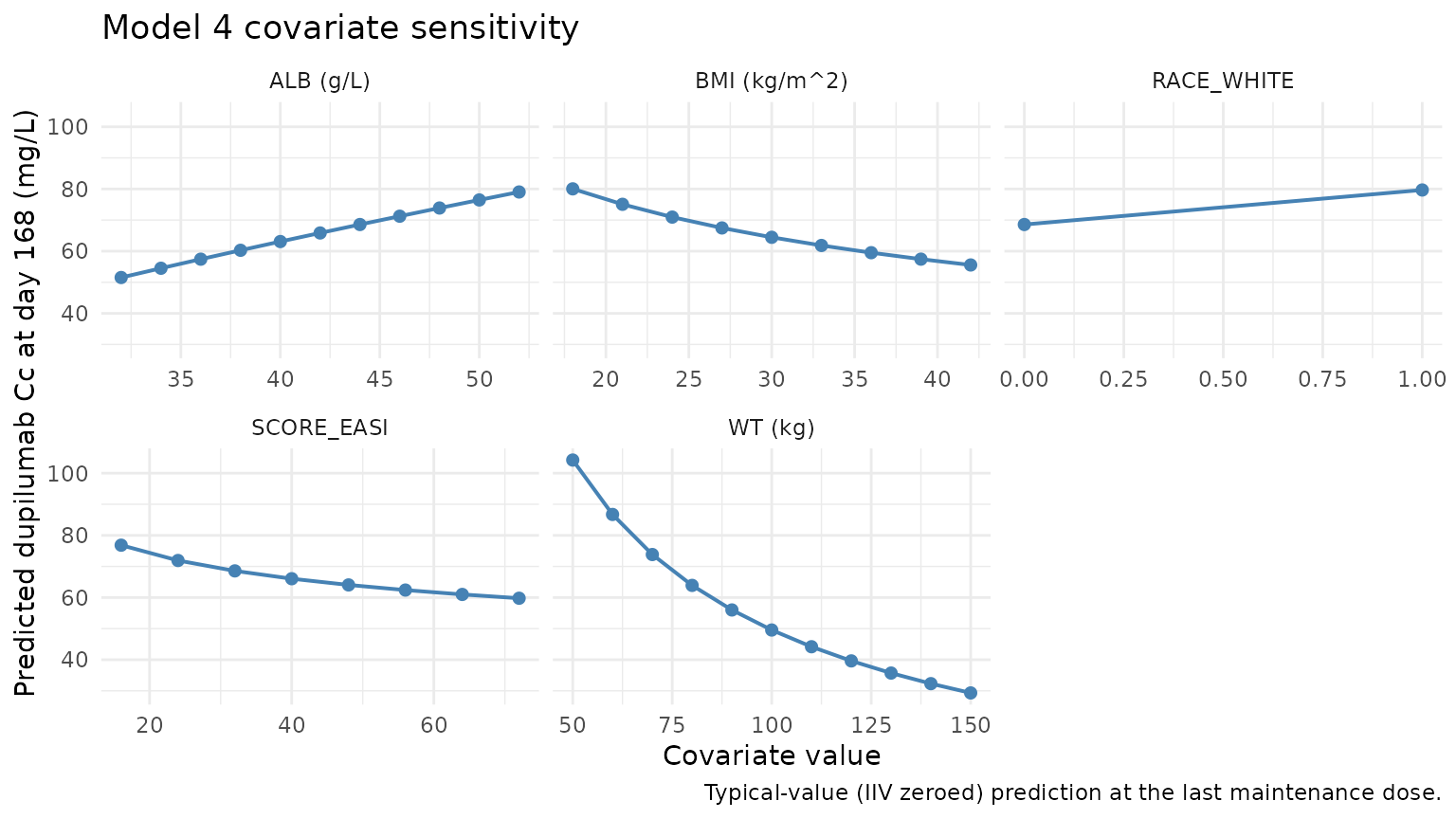
PKNCA validation
Non-compartmental analysis (NCA) of the steady-state Q2W interval (days 168-182) across the three packaged models. For each model, compute Cmax, Cmin (trough at end of tau), AUC over tau, and average concentration per simulated subject; compare the median across subjects against the others to confirm that Models 3 and 4 give similar typical-subject exposures and that Model 1’s rich-data parameterisation is broadly consistent.
ss_start <- tau * n_maint # day 168 (time of dose 13)
ss_end   <- ss_start + tau # day 182

pknca_per_model <- function(sim_df, model_label) {
  nca_conc <- sim_df |>
    dplyr::filter(time >= ss_start, time <= ss_end, !is.na(Cc)) |>
    dplyr::mutate(time_nom = time - ss_start, treatment = model_label) |>
    dplyr::select(id, time = time_nom, Cc, treatment)

  # Guarantee a time=0 row per (id, treatment); for extravascular pre-dose
  # the steady-state trough is the right anchor, but the AUC interval begins
  # at the dosing event, where Cc just after dose 13 == Cc just before
  # dose 14.  Defensively bind a Cc(0) row using the first available
  # observation per subject; PKNCA's AUC routines need a t=0 anchor.
  first_per_id <- nca_conc |>
    dplyr::group_by(id, treatment) |>
    dplyr::slice_min(time, n = 1L, with_ties = FALSE) |>
    dplyr::ungroup() |>
    dplyr::mutate(time = 0)
  nca_conc <- dplyr::bind_rows(nca_conc, first_per_id) |>
    dplyr::distinct(id, treatment, time, .keep_all = TRUE) |>
    dplyr::arrange(id, treatment, time)

  nca_dose <- cohort |>
    dplyr::mutate(time = 0, amt = maint_dose, treatment = model_label) |>
    dplyr::select(id, time, amt, treatment)

  conc_obj <- PKNCA::PKNCAconc(nca_conc, Cc ~ time | treatment + id)
  dose_obj <- PKNCA::PKNCAdose(nca_dose, amt ~ time | treatment + id)

  intervals <- data.frame(
    start   = 0,
    end     = tau,
    cmax    = TRUE,
    cmin    = TRUE,
    auclast = TRUE,
    cav     = TRUE
  )

  PKNCA::pk.nca(PKNCA::PKNCAdata(conc_obj, dose_obj, intervals = intervals))
}

nca_m1 <- pknca_per_model(sim_m1, "Model 1 (rich-data fit)")
nca_m3 <- pknca_per_model(sim_m3, "Model 3 (Phase 3 base)")
nca_m4 <- pknca_per_model(sim_m4, "Model 4 (Phase 3 covariate)")
summary(nca_m4)
#>  start end                   treatment   N     auclast       cmax        cmin
#>      0  14 Model 4 (Phase 3 covariate) 200 1280 [41.8] 101 [39.8] 76.6 [45.7]
#>          cav
#>  91.3 [41.8]
#>
#> Caption: auclast, cmax, cmin, cav: geometric mean and geometric coefficient of variation; N: number of subjects
Typical-subject steady-state exposure (cross-model comparison)
Kovalenko 2020 does not tabulate point estimates for steady-state Cmax, Ctrough, or AUC_tau in the main text; Figure 5 shows simulated medians qualitatively, and dupilumab FDA labelling reports typical steady-state trough concentrations of ~70-80 mg/L for a 75-kg adult on the 600-mg-load + 300-mg-Q2W SC regimen. The typical-value (“population typical”) prediction with IIV zeroed out provides a direct cross-model self-consistency check.
typical_one <- function(mod, model_label) {
  mod_typ <- mod |> rxode2::zeroRe()
  ev_typical <- events |>
    dplyr::filter(id == 1L) |>
    dplyr::mutate(WT = 75, ALB = 44, BMI = 26, SCORE_EASI = 32, RACE_WHITE = 0L)
  sim_typ <- rxode2::rxSolve(mod_typ, events = ev_typical) |> as.data.frame()
  ss_typ <- sim_typ |>
    dplyr::filter(time >= ss_start, time <= ss_end, !is.na(Cc))
  tibble::tibble(
    model              = model_label,
    Cmax_mgL           = max(ss_typ$Cc),
    Ctrough_mgL        = min(ss_typ$Cc),
    Cavg_mgL           = mean(ss_typ$Cc),
    AUCtau_day_mgL     = sum(diff(ss_typ$time) *
                             (ss_typ$Cc[-length(ss_typ$Cc)] +
                              ss_typ$Cc[-1]) / 2)
  )
}

typical_summary <- dplyr::bind_rows(
  typical_one(mod_m1, "Model 1 (rich-data fit)"),
  typical_one(mod_m3, "Model 3 (Phase 3 base)"),
  typical_one(mod_m4, "Model 4 (Phase 3 covariate)")
)
#> ℹ omega/sigma items treated as zero: 'etalvc', 'etalkel', 'etalka', 'etalvmax', 'etalmtt'
#> ℹ omega/sigma items treated as zero: 'etalvc', 'etalkel'
#> ℹ omega/sigma items treated as zero: 'etalvc', 'etalkel'
knitr::kable(typical_summary, digits = 2,
  caption = paste0("Typical-subject steady-state exposure ",
                   "(WT 75 kg, ALB 44 g/L, BMI 26 kg/m^2, ",
"SCORE_EASI 32, RACE_WHITE = 0; IIV zeroed)."))| model | Cmax_mgL | Ctrough_mgL | Cavg_mgL | AUCtau_day_mgL |
|---|---|---|---|---|
| Model 1 (rich-data fit) | 92.79 | 70.04 | 82.26 | 1173.27 |
| Model 3 (Phase 3 base) | 96.34 | 73.02 | 85.39 | 1217.03 |
| Model 4 (Phase 3 covariate) | 91.99 | 68.57 | 80.96 | 1155.14 |
The three models give broadly consistent typical-subject steady-state exposures. Differences arise mainly from the change in linear elimination rate ke (Model 1: 0.0534 1/d; Model 3: 0.0448 1/d; Model 4: 0.0477 1/d at the typical reference patient). Models 3 and 4 are calibrated to the same Phase 3 cohort; Model 1 used the earlier rich Phase 1/2 data.
Assumptions and deviations
- Models 1, 3, and 4 are packaged separately because the authors developed them with distinct parameter-estimation scopes (rich data, Phase 3 base, Phase 3 covariate). Model 2 is not packaged separately because the only covariates tested (population, assay version) were not retained.
- The reference body weight (75 kg) is inherited from Kovalenko 2016 (doi:10.1002/psp4.12136); Kovalenko 2020 does not restate the reference weight. The same value is used for Models 1, 3, and 4.
- For Model 4, the reference covariate values for albumin (44 g/L),
BMI (26 kg/m^2), and SCORE_EASI (32) are NOT stated in Kovalenko 2020.
The values adopted here are the closest published medians from sibling
analyses of the same Phase 3 dupilumab AD trials: ALB = 44 g/L matches
Zhang 2021 (doi:10.1002/psp4.12667) pooled dupilumab cohort; BMI and
EASI match LIBERTY AD SOLO 1/2 Simpson 2016 (Table 1) and CHRONOS
Blauvelt 2017 (Table 1). Users with access to a Phase 3 baseline
demographics table can re-scale by overriding these reference values in
the
model()block. - For the dichotomous race (White) covariate, the implementation form
ke * (1 + e_race_white_kel * RACE_WHITE)follows the Zhang 2021 dupilumab ADA-covariate precedent (same drug, same authorship group). The published theta = -0.123 implies a ~12% slower linear elimination rate for White subjects relative to the non-White reference. - IIV (omega) is reported in Kovalenko 2020 as a standard deviation,
per the Methods definition. Values in
ini()are squared to yield the variance that nlmixr2 stores with the~operator. Models 3 and 4 use a correlated(etalvc, etalkel)block; the covariance is computed inline in each model file’sini(). - The
etalmtteta in Model 1 is applied as log-normal on MTT (MTT = exp(lmtt + etalmtt)), whereas Supplementary Table S2 implements the random effect additively on MTT. The log-normal form prevents non-physical negative MTT draws during simulation. Models 3 and 4 do not have IIV on MTT (it is fixed), so this deviation does not apply. - Demographic details (age, sex, race breakdown) are not used by Models 1 or 3 (only WT enters the covariate model for Model 1, plus weight only for Model 3) and so are not exercised in the virtual cohort beyond the RACE_WHITE indicator that Model 4 requires.
- Kovalenko 2020 does not publish numerical Cmax / Cmin / AUC_tau at steady state, so the PKNCA summary and the typical-subject table above are cross-model self-consistency checks rather than back-to-paper numerical comparisons.
- No unit conversion is required between the dosing amount (mg) and
the concentration unit (mg/L) because mg/L is the natural unit of
central/vchere for all three models. - No erratum or correction notice was identified for Kovalenko 2020 at the time of this extraction; if one is published the per-parameter source-trace comments should be updated to point to the erratum.