Peginterferon alfa-2b (Gupta 2006)
Source:vignettes/articles/Gupta_2006_peginterferon_alfa_2b.Rmd
Gupta_2006_peginterferon_alfa_2b.RmdModel and source
- Citation: Gupta S, Jen J, Kolz K, Cutler D. Dose selection and population pharmacokinetics of PEGIntron in patients with chronic myelogenous leukaemia. Br J Clin Pharmacol. 2006;63(3):292-299. doi:10.1111/j.1365-2125.2006.02757.x
- Description: One-compartment population PK model with first-order subcutaneous absorption for peginterferon alfa-2b (PEG-Intron) in adult patients with chronic myelogenous leukaemia (Gupta 2006). Apparent clearance declines over treatment time via an Emax-type function CL(t) = CL0 / (1 + (t / T50)^beta) with beta fixed to 1 in the final model, so CL(t) = CL0 / (1 + t / T50). Cockcroft-Gault creatinine clearance modifies baseline clearance via a power form. Exponential IIV on CL0, T50, and V; proportional residual error on plasma concentration.
- Article: Br J Clin Pharmacol. 2006;63(3):292-299
Population
Gupta 2006 enrolled 137 adults (59 female / 78 male; 43.1% female) with newly diagnosed chronic-phase chronic myelogenous leukaemia (CML) in a randomised, multicentre, open-label, parallel-group Phase II/III trial of PEG-Intron versus INTRON A. Baseline demographics (Gupta 2006 Table 1): age 51 years (range 20-75), body weight 74.3 kg (42-137), serum creatinine 0.8 mg/dL (0.4-1.1, all within the normal range), Cockcroft-Gault creatinine clearance 113 mL/min (53-223; the published unit “ml h-1” in Table 1 is a typesetting error – the values are mL/min, consistent with Table 3 footer’s “CLcr 120 ml min-1”). Race distribution: 115 (83.9%) White, 3 (2.2%) Black, 19 (13.9%) Other. The international cohort (n = 111) dominated the US cohort (n = 26).
PEG-Intron was administered subcutaneously once weekly at an initial dose of 6.0 ug/kg/week with allowed dose reductions to 4.5 or 3.0 ug/kg/week (and discontinuation) based on individual tolerability; treatment continued up to a maximum of 48 weeks. The PK analysis used 624 serum PEG-Intron concentrations collected as pre-dose troughs at treatment weeks 4, 12, 24, 36, and 48 plus single post-dose samples on weeks 12 (24 h), 24 (72 h), and 36 (120 h).
The same information is available programmatically via
readModelDb("Gupta_2006_peginterferon_alfa_2b")$population.
Source trace
Per-parameter origin is recorded as an in-file comment next to each
ini() entry in
inst/modeldb/specificDrugs/Gupta_2006_peginterferon_alfa_2b.R.
The table below collects them for review.
| Equation / parameter | Value | Source location |
|---|---|---|
lcl |
log(44.1) L/day at CLcr 120 mL/min |
Gupta 2006 Table 3 (theta_CL0) |
lt50 |
log(23.8 * 28) = log(666.4) days |
Gupta 2006 Table 3 (theta_T50 in 28-day units) |
lvc |
log(149) L |
Gupta 2006 Table 3 (V) |
lka (fixed) |
log(1.9) 1/day |
Gupta 2006 Table 3 (Ka, FIXED at Phase I CHC mean per refs 9-10) |
e_crcl_cl |
0.21 |
Gupta 2006 Table 3 (theta_CLcr) |
etalcl IIV |
0.1156 (CV 35%) |
Gupta 2006 Table 3 (omega(CV) CL0) ->
omega^2 = log(0.35^2 + 1)
|
etalt50 IIV |
0.7833 (CV 109%) |
Gupta 2006 Table 3 (omega(CV) T50) ->
omega^2 = log(1.09^2 + 1)
|
etalvc IIV |
0.2986 (CV 59%) |
Gupta 2006 Table 3 (omega(CV) V) ->
omega^2 = log(0.59^2 + 1)
|
propSd |
0.414 (proportional CV 41.4%) |
Gupta 2006 Table 3 (sigma_epsilon = 41.4; see Errata) |
| CL covariate form | CL0 = 44.1 * (CRCL / 120)^0.21 * exp(eta_CL0) |
Gupta 2006 Methods covariate equation |
| Time-varying CL |
CL(t) = CL0 / (1 + (t / T50)^beta), beta = 1 fixed |
Gupta 2006 Methods Emax-type decline; final model |
| One-compartment ODEs |
d depot/dt = -Ka depot;
d central/dt = Ka depot - (CL/V) central;
Cc = central/V
|
Gupta 2006 Methods (one-compartment first-order absorption + elimination) |
| Residual error form | Y = Cc * (1 + eps_prop) |
Gupta 2006 Table 3 sigma_epsilon = 41.4 interpreted as proportional CV (see Errata) |
Virtual cohort
The Gupta 2006 patient-level data are not publicly available. The cohort below samples baseline body weight and Cockcroft-Gault creatinine clearance from log-normal distributions whose location and spread approximate the cohort summary statistics in Gupta 2006 Table 1 (WT mean 74.3 kg, range 42-137; CRCL mean 113 mL/min, range 53-223). The race distribution mirrors Table 1 proportions (84% White, 2% Black, 14% Other); race is not used by the structural model (Gupta 2006 Table 2 Model 7: deltaOFV = 1.858, p = 0.173, not retained), so it is carried as a label only.
set.seed(20260606)
n_subjects <- 200L

make_lognormal <- function(mu, sd, n) {
  s    <- sqrt(log(1 + (sd / mu)^2))
  mlog <- log(mu) - 0.5 * s^2
  exp(rnorm(n, mean = mlog, sd = s))
}

# Approximate SDs from Table 1 ranges via (max - min) / 4 (4 SDs of a normal
# span ~95% of values; this is a coarse but conservative imputation when only
# range is reported).
wt_mean <- 74.3; wt_sd <- (137 - 42) / 4
cr_mean <- 113;  cr_sd <- (223 - 53) / 4

cohort <- tibble::tibble(
  id   = seq_len(n_subjects),
  WT   = pmin(pmax(make_lognormal(wt_mean, wt_sd, n_subjects), 42), 137),
  CRCL = pmin(pmax(make_lognormal(cr_mean, cr_sd, n_subjects), 53), 223)
)

# 6.0 ug/kg/week SC for 48 weeks (the primary PEG-Intron regimen in Gupta 2006).
# Dose in ug (the unit used by the source paper); the model converts internally
# to ng/mL by Cc = central / vc when dose is in ug and V is in L.
dose_per_kg_ug <- 6.0
doses <- cohort |>
  tidyr::crossing(dose_week = 0:47) |>
  dplyr::mutate(
    time = dose_week * 7,
    amt  = dose_per_kg_ug * WT,
    cmt  = "depot",
    evid = 1L
  ) |>
  dplyr::select(id, time, amt, cmt, evid, WT, CRCL)

# Observation grid: dense around each dose to characterise SC absorption peak,
# plus a coarse grid over the 48-week treatment period.
post_dose_grid <- c(0, 0.25, 0.5, 1, 1.5, 2, 3, 4, 5, 6, 7) # days post each weekly dose
obs_grid_days  <- sort(unique(c(
  seq(0, 7 * 48, by = 7),                                              # weekly trough envelope
  unlist(lapply(c(4, 12, 24, 36, 48), function(wk) (wk - 1) * 7 + post_dose_grid))
)))

obs <- cohort |>
  tidyr::crossing(time = obs_grid_days) |>
  dplyr::mutate(amt = 0, cmt = NA_character_, evid = 0L) |>
  dplyr::select(id, time, amt, cmt, evid, WT, CRCL)

events <- dplyr::bind_rows(doses, obs) |>
  dplyr::arrange(id, time, dplyr::desc(evid))

stopifnot(!anyDuplicated(events[, c("id", "time", "evid", "amt")]))
Simulation
mod <- rxode2::rxode(readModelDb("Gupta_2006_peginterferon_alfa_2b"))
#> ℹ parameter labels from comments will be replaced by 'label()'

sim <- rxode2::rxSolve(mod, events = events, keep = c("WT", "CRCL")) |>
  as.data.frame() |>
  tibble::as_tibble()
Replicate published behavior
Time-varying apparent clearance (replicates Figure 4 of Gupta 2006)
Gupta 2006 Figure 4 shows the population-mean PEG-Intron apparent
clearance declining smoothly over the 48-week treatment period (CML
solid line plus three chronic hepatitis C broken lines from earlier
studies). With the typical parameters held fixed (zeroRe())
and CRCL set to the reference 120 mL/min, the model’s clearance
trajectory is the closed form
CL(t) = 44.1 / (1 + t / 666.4) L/day. The plot below
evaluates it at the points Gupta 2006 highlights – weeks 4 (42.3 L/day)
and 48 (29.3 L/day) – and confirms a 30.8% reduction in clearance from
week 4 to week 48.
typical_cl <- function(t_days, cl0 = 44.1, t50 = 666.4) cl0 / (1 + t_days / t50)

cl_traj <- tibble::tibble(
  day    = seq(0, 7 * 48, length.out = 200),
  cl_pred = typical_cl(day)
) |>
  dplyr::mutate(week = day / 7)

cl_marks <- tibble::tibble(
  week   = c(4, 48),
  day    = week * 7,
  cl_pub = c(42.3, 29.3),
  label  = sprintf("Week %d: published %.1f L/day", week, cl_pub)
)

ggplot(cl_traj, aes(week, cl_pred)) +
  geom_line(linewidth = 0.8) +
  geom_point(data = cl_marks, aes(week, cl_pub),
             colour = "red", size = 3) +
  geom_text(data = cl_marks, aes(week, cl_pub, label = label),
            colour = "red", hjust = -0.05, vjust = -1, size = 3) +
  labs(x = "Treatment week", y = "Apparent CL (L/day)",
       title = "Replicates Figure 4 of Gupta 2006 (CML solid line)",
       caption = "Solid line: typical CL trajectory. Red points: published mean CL at weeks 4 and 48.")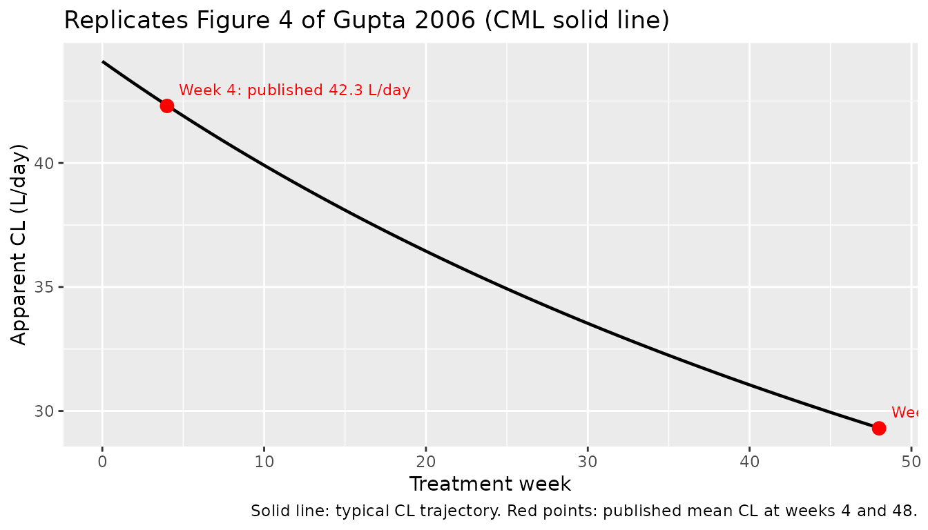
# Numerical reproduction
reduction_pct <- 100 * (typical_cl(28) - typical_cl(336)) / typical_cl(28)
data.frame(
  week_4_pred_L_per_day  = round(typical_cl(28), 2),
  week_48_pred_L_per_day = round(typical_cl(336), 2),
  reduction_pct          = round(reduction_pct, 1)
)
#>   week_4_pred_L_per_day week_48_pred_L_per_day reduction_pct
#> 1                 42.32                  29.32          30.7
Concentration profiles by treatment week (replicates Figure 1 of Gupta 2006)
Gupta 2006 Figure 1 plots immunoassay concentrations versus elapsed
time from the previous dose, broken out by treatment week (4, 12, 24,
36, 48). The plot below shows the simulated 5-50-95 percentile envelope
of Cc over the 0-7 day post-dose window for each of those
weeks, with concentrations converted from ng/mL to
pg/mL (1 ng/mL = 1000 pg/mL) to match the published y-axis
units.
weeks_to_show <- c(4, 12, 24, 36, 48)

window <- sim |>
  dplyr::mutate(week = time / 7) |>
  dplyr::filter(week >= 3, week <= 48) |>
  dplyr::mutate(
    dose_week     = floor((week - 1) / 1) + 1,
    sample_week   = floor(week),
    elapsed_days  = time - (sample_week - 1) * 7
  ) |>
  dplyr::filter(sample_week %in% weeks_to_show, elapsed_days >= 0, elapsed_days <= 7) |>
  dplyr::group_by(sample_week, elapsed_days) |>
  dplyr::summarise(
    Cc_pg_per_mL_Q05 = quantile(Cc * 1000, 0.05, na.rm = TRUE),
    Cc_pg_per_mL_Q50 = quantile(Cc * 1000, 0.50, na.rm = TRUE),
    Cc_pg_per_mL_Q95 = quantile(Cc * 1000, 0.95, na.rm = TRUE),
    .groups = "drop"
  )

ggplot(window, aes(elapsed_days, Cc_pg_per_mL_Q50)) +
  geom_ribbon(aes(ymin = Cc_pg_per_mL_Q05, ymax = Cc_pg_per_mL_Q95), alpha = 0.25) +
  geom_line(linewidth = 0.8) +
  facet_wrap(~ paste("Week", sample_week)) +
  labs(x = "Elapsed time after dose (days)", y = "Cc (pg/mL)",
       title = "Replicates Figure 1 of Gupta 2006: Cc vs. elapsed time, by treatment week",
       caption = "Shaded band: 5-95th percentile of the simulated cohort; solid line: median.")
#> `geom_line()`: Each group consists of only one observation.
#> ℹ Do you need to adjust the group aesthetic?
#> `geom_line()`: Each group consists of only one observation.
#> ℹ Do you need to adjust the group aesthetic?
#> `geom_line()`: Each group consists of only one observation.
#> ℹ Do you need to adjust the group aesthetic?
#> `geom_line()`: Each group consists of only one observation.
#> ℹ Do you need to adjust the group aesthetic?
#> `geom_line()`: Each group consists of only one observation.
#> ℹ Do you need to adjust the group aesthetic?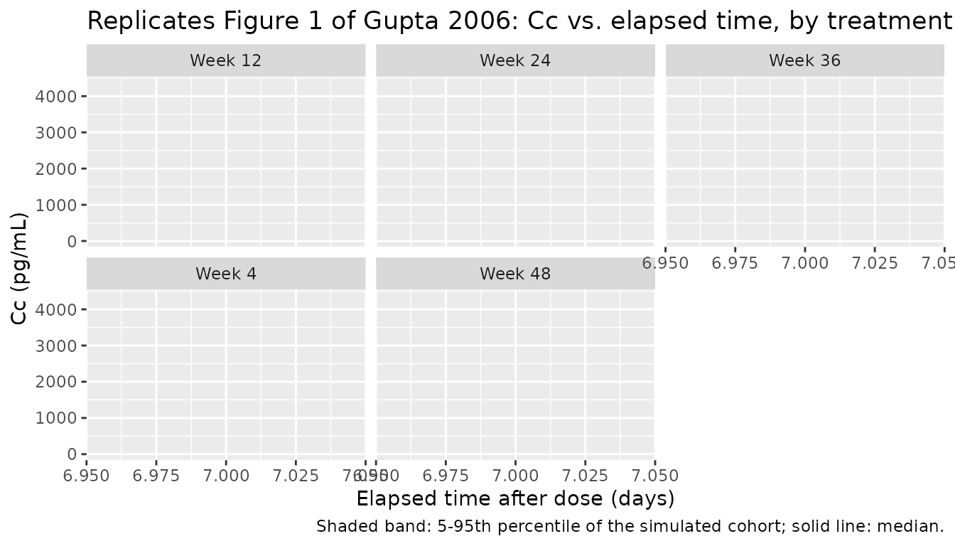
Typical-value Tmax sanity check
For a single dose with first-order absorption and first-order
elimination, the typical-value Tmax is
log(ka / kel) / (ka - kel). Using the Table 3 point
estimates at t = 0 (so CL = CL0) and CRCL = 120 mL/min:
ka  <- 1.9
cl0 <- 44.1
v   <- 149
kel0 <- cl0 / v
tmax_day  <- log(ka / kel0) / (ka - kel0)
tmax_hour <- tmax_day * 24
round(c(tmax_day = tmax_day, tmax_hour = tmax_hour), 2)
#>  tmax_day tmax_hour
#>      1.16     27.82
The closed-form Tmax (~1.16 days, ~28 h) is consistent with the published absorption profile (Gupta 2006 Figure 1 shows concentration peaks within the first 24-72 h after dosing).
PKNCA validation
We compute single-dosing-interval NCA over the week-4 and week-48
dosing intervals (days 21-28 and days 329-336 respectively) and compare
the AUC-derived apparent clearance against the published values (42.3
L/day at week 4, 29.3 L/day at week 48; Gupta 2006 Results).
Concentrations are kept in ng/mL so that
dose (ug) / AUC (ng*day/mL) gives clearance in
L/day via the identity
1 ug / 1 ng/mL = 1 L.
# Build a PKNCA conc + dose data set restricted to two intervals.
# Each interval is one weekly dose followed by a 7-day observation window.
make_interval_data <- function(sim_data, ev_data, week, label) {
  start_day <- (week - 1) * 7
  end_day   <- week * 7

  conc <- sim_data |>
    dplyr::filter(time >= start_day, time <= end_day, !is.na(Cc)) |>
    dplyr::mutate(time_in_interval = time - start_day, treatment = label) |>
    dplyr::select(id, time_in_interval, Cc, treatment) |>
    dplyr::rename(time = time_in_interval)

  conc <- dplyr::bind_rows(
    conc,
    conc |> dplyr::distinct(id, treatment) |>
      dplyr::mutate(time = 0, Cc = 0)
  ) |>
    dplyr::distinct(id, treatment, time, .keep_all = TRUE) |>
    dplyr::arrange(id, treatment, time)

  dose <- ev_data |>
    dplyr::filter(evid == 1L, time == start_day) |>
    dplyr::mutate(treatment = label, time = 0) |>
    dplyr::select(id, time, amt, treatment)

  list(conc = conc, dose = dose)
}

iv_wk4  <- make_interval_data(sim, events, week = 4,  label = "Week 4 (6 ug/kg/week)")
iv_wk48 <- make_interval_data(sim, events, week = 48, label = "Week 48 (6 ug/kg/week)")

conc_all <- dplyr::bind_rows(iv_wk4$conc, iv_wk48$conc)
dose_all <- dplyr::bind_rows(iv_wk4$dose, iv_wk48$dose)

conc_obj <- PKNCA::PKNCAconc(conc_all, Cc ~ time | treatment + id,
                             concu = "ng/mL", timeu = "day")
dose_obj <- PKNCA::PKNCAdose(dose_all, amt ~ time | treatment + id,
                             doseu = "ug")

intervals <- data.frame(
  start      = 0,
  end        = 7,
  cmax       = TRUE,
  tmax       = TRUE,
  auclast    = TRUE,
  cl.last    = TRUE
)

nca_res <- PKNCA::pk.nca(PKNCA::PKNCAdata(conc_obj, dose_obj,
                                          intervals = intervals))

nca_summary <- as.data.frame(nca_res$result) |>
  dplyr::filter(PPTESTCD %in% c("cmax", "tmax", "auclast", "cl.last")) |>
  dplyr::group_by(treatment, PPTESTCD) |>
  dplyr::summarise(median = stats::median(PPORRES, na.rm = TRUE),
                   q05    = stats::quantile(PPORRES, 0.05, na.rm = TRUE),
                   q95    = stats::quantile(PPORRES, 0.95, na.rm = TRUE),
                   .groups = "drop")

knitr::kable(nca_summary,
             digits = 3,
caption = "Simulated single-interval NCA at weeks 4 and 48 (6 ug/kg/week SC).")| treatment | PPTESTCD | median | q05 | q95 |
|---|---|---|---|---|
| Week 4 (6 ug/kg/week) | auclast | 10.935 | 4.725 | 23.494 |
| Week 4 (6 ug/kg/week) | cl.last | 40.394 | 22.612 | 71.383 |
| Week 4 (6 ug/kg/week) | cmax | 2.691 | 1.330 | 5.352 |
| Week 4 (6 ug/kg/week) | tmax | 1.000 | 1.000 | 1.500 |
| Week 48 (6 ug/kg/week) | auclast | 18.077 | 7.058 | 40.919 |
| Week 48 (6 ug/kg/week) | cl.last | 25.431 | 11.350 | 49.718 |
| Week 48 (6 ug/kg/week) | cmax | 3.717 | 1.685 | 7.666 |
| Week 48 (6 ug/kg/week) | tmax | 1.000 | 1.000 | 1.500 |
Comparison against published apparent clearance
Gupta 2006 reports the typical apparent clearance at week 4 = 42.3
L/day and at week 48 = 29.3 L/day. The table below compares those
published values against the cohort-median cl.last (= dose
/ AUClast over the 7-day dosing interval) from the simulation.
published <- tibble::tibble(
  treatment = c("Week 4 (6 ug/kg/week)", "Week 48 (6 ug/kg/week)"),
  cl.last   = c(42.3, 29.3)
)

cmp <- nlmixr2lib::ncaComparisonTable(
  simulated     = nca_res,
  reference     = published,
  by            = "treatment",
  params        = "cl.last",
  units         = c(cl.last = "L/day"),
  tolerance_pct = 20
)
#> Warning: ncaParamLabel(): unknown PKNCA code(s) returned as-is: 'cl.last'

knitr::kable(cmp,
             caption = paste(
               "Simulated cohort-median apparent clearance (cohort-median",
               "cl.last from PKNCA) vs. published mean CL at weeks 4 and 48",
               "(Gupta 2006 Results). * differs from reference by >20%."
             ),
align = c("l", "l", "r", "r", "r"))| NCA parameter | treatment | Reference | Simulated | % diff |
|---|---|---|---|---|
| cl.last (L/day) | Week 4 (6 ug/kg/week) | 42.3 | 40.4 | -4.5% |
| cl.last (L/day) | Week 48 (6 ug/kg/week) | 29.3 | 25.4 | -13.2% |
Assumptions and deviations
Residual error parameterisation (interpretation of Table 3 sigma_epsilon). Gupta 2006 Table 3 reports a single residual term
sigma_epsilon = 41.4 +/- 84.2%with a header unit(l day-1)that is a typesetting artifact (the residual is not a clearance; the published unit appears to be copied from the theta_CL0 row above). The Methods text describes a combined “multiplicative + additive” error model, but only one residual value is tabulated. We encode the 41.4 value as a proportional residual CV of 41.4% (propSd = 0.414) on plasma concentration; the 84.2% is interpreted as the relative standard error on the estimate (high RSE reflects the sparse- sampling design). This is the interpretation that is dimensionally consistent with the ECL immunoassay reporting in pg/mL (LLOQ 50 pg/mL, assay CV 12%, linear range 50-2000 pg/mL) and with sparsely-sampled popPK practice for this drug class (cf. Bi 2017 peginterferon alfa-2a, which reports residual proportional CV = 19.4% and additive SD = 0.32 ng/L). Downstream users who need a different residual structure should overridepropSdand/or add anaddSdterm.Cockcroft-Gault creatinine clearance reference and units. Gupta 2006 Table 1 lists CLcr as “ml h-1” with cohort range 53-223; Table 3 describes the reference patient as “CLcr 120 ml min-1”. The values themselves are in mL/min (a CLcr of 113 mL/h would correspond to a profoundly anuric adult, which is inconsistent with the cohort eligibility criteria). The model uses the canonical
CRCLcovariate column in mL/min with a reference value of 120 mL/min, matching the Table 3 footer.Time-varying clearance and “elapsed time” definition. The Methods section states
tis “the elapsed time in days relative to the treatment starting day”. In the model filetis the rxode2 / nlmixr2timevariable measured from the first event. As long as the events file places the first dose attime = 0and time is measured in days (the model’s declared time unit),timematches the paper’st.Beta fixed to 1. The final-model
beta(steepness parameter of the Emax-type clearance decline) was fixed at 1 in Gupta 2006 to avoid numerical difficulties (Results, “Covariate analysis and final model”). The model file encodes this simplification analytically –betadoes not appear as a parameter; the time-varying-CL equation reduces toCL(t) = CL0 / (1 + t / T50). A sensitivity analysis in the source paper showed +/- 20% perturbations of the fixedbetaandKaproduced little change in the other parameter estimates.IIV on V is in Table 3 but not in the Methods text. The Methods section enumerates only
eta_CL0andeta_T50as random effects, but Table 3 reportsomega(CV) = 59%for V. The model file follows Table 3 and carries an IIV term on V.Race covariate. Gupta 2006 Table 2 (Model 7) screened a binary RACE_OTHER indicator (1 = Black or Other, 0 = White; the paper pools the 3 Black and 19 Other patients into a single “other” category for fitting purposes). Race was not retained in the final model (deltaOFV = 1.858, p = 0.173). The screened covariates (WT, AGE, SEXF, CREAT, RACE_OTHER) are documented in
covariatesDataExcludedso a user assembling a virtual cohort knows what was tested but not retained.Cohort imputation for body weight and CRCL. Gupta 2006 Table 1 reports only mean and range for continuous covariates; SDs are not tabulated. The virtual cohort approximates SDs from the range via the heuristic
(max - min) / 4, which is a coarse but conservative imputation when only the cohort range is reported. The structural model has no body-weight covariate effect, so the WT distribution affects only the per-subject weight-based dose; CRCL enters the model directly via the(CRCL/120)^0.21scaling on CL0.Dose normalisation. The simulated cohort dose is the protocol-recommended 6.0 ug/kg/week throughout the 48-week treatment course. Gupta 2006 permitted protocol-defined dose reductions to 4.5 or 3.0 ug/kg/week based on individual tolerability; the simulation does not model the time-varying dose reductions, which would require subject-level adverse-event data that the publication does not provide.
Race / sex distribution not used by the structural model. Race is carried in
population$race_ethnicityfor documentation but the structural model has no race effect; the virtual cohort does not need a race column to drive any simulation output.