Model and source
- Citation: Watt KM, Thompson EJ, Lam L, Zimmerman K, Hornik CP, Atz AM, Fernandez A, Hupp SR, Bhatt-Mehta V, Benjamin DK Jr, Anand R, Cohen-Wolkowiez M, Gonzalez D, Smith PB, Capparelli EV; Best Pharmaceuticals for Children Act - Pediatric Trials Network Steering Committee. Population Pharmacokinetics to Support Intravenous and Enteral Methadone Dosing in Children. J Clin Pharmacol. 2026;66(1):e70143. doi:10.1002/jcph.70143
- Description: One-compartment population PK model of methadone in hospitalized children from birth to 21 years given intravenous or enteral methadone per standard of care for pain or iatrogenic opiate withdrawal (Watt 2026). First-order enteral absorption with ka fixed at 2.72 1/h, enteral bioavailability 0.64, allometric total-body-weight scaling on CL (exponent 0.75) and linear total-body-weight scaling on V (exponent 1) with both exponents fixed and NO weight normalization (the published equations scale raw kg, so CL = 0.325 * WT^0.75 = 7.87 L/h and V = 5.22 * WT = 365 L at 70 kg), correlated interindividual variability on CL and V, and proportional residual error. Body weight is the only covariate: the univariate screen flagged total bilirubin, serum creatinine and obesity on CL and postnatal age and total bilirubin on V, none survived backward elimination, fat-free mass performed no better than total body weight, and postnatal- / postmenstrual-age maturation functions did not improve the fit, so the base model is also the final irreducible model.
- Article: https://doi.org/10.1002/jcph.70143
- Supplement (Tables S1-S2, Figures S1-S6): published with the
open-access article (
PMC12755061).
Methadone concentrations in this vignette are reported in
ng/mL to match the paper. The packaged model works in
mg and L, so Cc is in mg/L and every display below
multiplies by 1000.
NG_PER_MG <- 1000              # Cc is mg/L; the paper reports ng/mL
TAU       <- 8                 # q8h in every simulated regimen
TARGET_PAIN <- 30              # ng/mL, Cmin target for pain control
TARGET_TOX  <- 300             # ng/mL, Cmax safety threshold
TARGET_AUC  <- 816             # ng*h/mL, AUC0-tau target to prevent withdrawal
DOSE_CAP_MG <- 10              # maximum 10 mg per dose
Population
The model was fit to 263 analyzable plasma methadone concentrations from 99 hospitalized children pooled across two prospective, multi-center, open-label Pediatric Trials Network studies conducted at 23 US children’s hospitals (Watt 2026 Table 1): MTH01 (NCT01945736, 5 sites, n = 26, scheduled sampling after multiple enteral doses in children >= 90 days to < 18 years treated for iatrogenic opiate withdrawal) and POPS (NCT01431326, 18 sites, n = 73, opportunistic standard-of-care sampling in children < 21 years).
Median (range) postnatal age was 2.29 (0-19.02) years and weight 13.0 (0.72-159.0) kg; 49/99 (50%) were male; 72% White, 20% Black or African American, 6% multiple races, 1% Asian, and 13 participants (19% of those reporting ethnicity) Hispanic or Latino. Forty-four children (44%) were younger than 2 years and so, per CDC guidance, could not be classified for obesity; among the remaining 55, 22 were obese. Of 1798 recorded doses 232 (13%) were intravenous; 10 participants received only IV doses, 78 only enteral doses, and 11 both. Median (range) weight-normalized doses were 0.11 (0.01-0.39) mg/kg IV and 0.10 (0.01-0.61) mg/kg enterally. Samples were drawn a median 4 h (0-31.8) after the last dose and the median (range) concentration was 42.2 (0.9-729.2) ng/mL, all within the 0.1-100 ng/mL validated assay range after dilution. Laboratory covariates were split by protocol: alpha-1-acid glycoprotein, hematocrit and CYP genotypes in MTH01 only; albumin, ALT, AST, serum creatinine and total bilirubin in POPS only.
The same information is available programmatically:
pop <- rxode2::rxode(readModelDb("Watt_2026_methadone"))$population
#> ℹ parameter labels from comments will be replaced by 'label()'
str(pop, max.level = 1)
#> List of 13
#>  $ species       : chr "human"
#>  $ n_subjects    : int 99
#>  $ n_studies     : int 2
#>  $ age_range     : chr "0-19.02 years (postnatal age); eligibility birth to < 21 years"
#>  $ age_median    : chr "2.29 years"
#>  $ weight_range  : chr "0.72-159.0 kg"
#>  $ weight_median : chr "13.0 kg"
#>  $ sex_female_pct: num 50.5
#>  $ race_ethnicity: Named num [1:5] 72 20 1 6 1
#>   ..- attr(*, "names")= chr [1:5] "White" "Black" "Asian" "Multiple" ...
#>  $ disease_state : chr "Hospitalized children prescribed methadone per standard of care for pain or iatrogenic opiate withdrawal"
#>  $ dose_range    : chr "IV 0.11 (0.01-0.39) mg/kg and enteral 0.10 (0.01-0.61) mg/kg per dose, median (range); 1798 recorded doses of w"| __truncated__
#>  $ regions       : chr "USA (23 enrolling children's hospitals)"
#>  $ notes         : chr "Pooled from two prospective, multi-center, open-label PK studies (Watt 2026 Table 1): MTH01 (NCT01945736, 5 sit"| __truncated__
Source trace
Every ini() entry in
inst/modeldb/specificDrugs/Watt_2026_methadone.R carries an
in-file comment naming its source location. They are collected here for
review.
| Equation / parameter | Value | Source location |
|---|---|---|
lcl (CL coefficient) |
0.325 L/h/kg^0.75 | Table 2, “CL (L/h/kg)”; %RSE 21.6; bootstrap 0.171-0.516 |
lvc (V coefficient) |
5.22 L/kg | Table 2, “V (L/kg)”; %RSE 21.8; bootstrap 2.70-8.01 |
lka |
2.72 1/h, fixed | Table 2, “KA (1/h) 2.72 FIX”; Equation 6 |
lfdepot |
0.64 | Table 2, “F”; %RSE 21.8; bootstrap 0.32-1.00; Equation 7 |
e_wt_cl |
0.75, fixed | Methods, Population Pharmacokinetic Analysis (“allometric scaling - WT^0.75”); Equation 5 |
e_wt_vc |
1.0, fixed | Methods, Population Pharmacokinetic Analysis (“linear scaling - WT^1.0”); Equation 4 |
etalcl variance |
0.881^2 = 0.7762 | Table 2, “CL interindividual variability (CV%)” 88.1 |
etalvc variance |
0.740^2 = 0.5476 | Table 2, “V interindividual variability (CV%)” 74.0 |
etalcl ~ etalvc covariance |
0.296 | Table 2, “CL ~ V interindividual variability covariance”; %RSE 34.5 |
propSd |
0.240 | Table 2, “Residual proportional error (CV%)” 24.0 |
V (L) = theta1 * WT |
n/a | Equation 4 |
CL (L/h) = theta2 * WT^0.75 |
n/a | Equation 5 |
d/dt(depot), d/dt(central),
f(depot)
|
n/a | Results, Population PK Model Development (one-compartment model with proportional residual error, first-order enteral absorption, bioavailability F on the enteral route) |
| No covariate effects | n/a | Results, Covariate Analysis (“Because no covariates were retained, the base model was used as the final irreducible model”) |
Structural checks against printed values
These are deterministic (typical-value) checks with no simulated cohort, so they can be asserted tightly.
Reference-weight clearance and volume
Watt 2026 restates its size model as “values for CL and V of 7.87 L/h/70 kg and 365 L/70 kg”. Because Equations 4-5 scale raw kilograms with no reference-weight divisor, this is a genuine external check on the encoding: a model that mistakenly normalized to 70 kg would return 0.325 L/h and 5.22 L here.
mod  <- readModelDb("Watt_2026_methadone")
modT <- rxode2::zeroRe(mod)
#> ℹ parameter labels from comments will be replaced by 'label()'

solve_typical <- function(wt, route = "central", amt = 1, times = c(0, 1)) {
  ev <- data.frame(
    id   = 1L,
    time = c(0, times),
    amt  = c(amt, rep(NA_real_, length(times))),
    evid = c(1L, rep(0L, length(times))),
    cmt  = c(route, rep("central", length(times))),
    WT   = wt
  )
  as.data.frame(rxode2::rxSolve(modT, ev, returnType = "data.frame"))
}

s70 <- solve_typical(70)
#> ℹ omega/sigma items treated as zero: 'etalcl', 'etalvc'
cl70 <- s70$cl[1]
vc70 <- s70$vc[1]

c(CL_70kg_Lh = cl70, V_70kg_L = vc70)
#> CL_70kg_Lh   V_70kg_L
#>   7.865148 365.400000

# Paper prints 7.87 and 365 (rounded to 3 significant figures).
stopifnot(
  abs(cl70 / 7.87 - 1) < 0.005,
  abs(vc70 / 365  - 1) < 0.005
)
Mass balance and enteral bioavailability
The ODE identity
AUC[0,T] * CL == (dose absorbed) - (amount still in the system)
holds exactly at any T, so it is a strong structural gate:
it would break if f(depot) were attached to the wrong
compartment, if the depot leaked, or if kel were
mis-derived. Running it for both routes also recovers F
independently of the ini() value, because the enteral-to-IV
AUC ratio for the same dose is exactly F.
tgrid <- seq(0, 480, by = 0.05)

mb <- lapply(c(central = "central", depot = "depot"), function(rt) {
  s <- solve_typical(wt = 20, route = rt, amt = 5, times = tgrid)
  auc <- sum(diff(s$time) * (head(s$Cc, -1) + tail(s$Cc, -1)) / 2)
  data.frame(
    route     = rt,
    auc_clr   = auc * s$cl[1],
    remaining = tail(s$central, 1) + tail(s$depot, 1),
    aucinf    = auc
  )
}) |> bind_rows()
#> ℹ omega/sigma items treated as zero: 'etalcl', 'etalvc'
#> ℹ omega/sigma items treated as zero: 'etalcl', 'etalvc'

f_recovered <- mb$aucinf[mb$route == "depot"] / mb$aucinf[mb$route == "central"]
f_ini       <- exp(rxode2::rxode(mod)$theta[["lfdepot"]])
#> ℹ parameter labels from comments will be replaced by 'label()'

c(F_from_AUC_ratio = f_recovered, F_from_ini = f_ini)
#> F_from_AUC_ratio       F_from_ini
#>        0.6399892        0.6400000

stopifnot(
  # Mass balance: AUC*CL recovers the absorbed dose minus what is left.
  all(abs(mb$auc_clr / (c(5, 5 * f_ini) - mb$remaining) - 1) < 1e-3),
  # The enteral/IV AUC ratio IS F, to solver tolerance.
  abs(f_recovered / f_ini - 1) < 1e-3,
  abs(f_ini - 0.64) < 1e-12
)
Post hoc parameters by age group (Table 3)
Watt 2026 Table 3 reports median empiric Bayes CL, CL/kg, V/kg and
half-life by age group. Because median(exp(eta)) = 1 for a
log-normal random effect, the typical-value prediction at each group’s
median weight should approximate the group’s post hoc median. Half-life
is the sharpest of these: it is log(2) * V/CL, which under
this size model is proportional to WT^0.25, so reproducing
it across a 2.8-90.6 kg span tests both exponents and the ratio of the
two coefficients at once.
tab3 <- tibble::tribble(
  ~group,                  ~wt,  ~cl_pub, ~clkg_pub, ~vkg_pub, ~thalf_pub,
  "<= 30 days",             2.8,  0.94,    0.27,      6.10,     15.8,
  "31 days to < 6 months",  4.4,  0.91,    0.20,      5.50,     15.0,
  "6 months to < 2 years",  9.8,  1.40,    0.17,      4.50,     19.1,
  "2 to < 13 years",       19.8,  3.90,    0.19,      5.49,     22.1,
  "13 to < 17 years",      90.6,  4.49,    0.047,     3.29,     40.4,
  "17 to < 21 years",      78.0, 10.48,    0.16,      3.35,     34.4,
  "Overall",               13.0,  2.97,    0.17,      4.99,     20.5
)

tab3 <- tab3 |>
  rowwise() |>
  mutate(
    .s     = list(solve_typical(wt)),
    cl_mod = .s$cl[1],
    vc_mod = .s$vc[1]
  ) |>
  ungroup() |>
  mutate(
    clkg_mod  = cl_mod / wt,
    vkg_mod   = vc_mod / wt,
    thalf_mod = log(2) * vc_mod / cl_mod,
    d_thalf   = 100 * (thalf_mod / thalf_pub - 1),
    d_clkg    = 100 * (clkg_mod  / clkg_pub  - 1),
    d_vkg     = 100 * (vkg_mod   / vkg_pub   - 1)
  ) |>
  select(-.s)
#> ℹ omega/sigma items treated as zero: 'etalcl', 'etalvc'
#> ℹ omega/sigma items treated as zero: 'etalcl', 'etalvc'
#> ℹ omega/sigma items treated as zero: 'etalcl', 'etalvc'
#> ℹ omega/sigma items treated as zero: 'etalcl', 'etalvc'
#> ℹ omega/sigma items treated as zero: 'etalcl', 'etalvc'
#> ℹ omega/sigma items treated as zero: 'etalcl', 'etalvc'
#> ℹ omega/sigma items treated as zero: 'etalcl', 'etalvc'

tab3 |>
  transmute(
    "Age group (PNA)"       = group,
    "Median weight (kg)"    = wt,
    "t1/2 published (h)"    = thalf_pub,
    "t1/2 model (h)"        = round(thalf_mod, 1),
    "t1/2 % diff"           = round(d_thalf, 1),
    "CL/kg published"       = clkg_pub,
    "CL/kg model"           = round(clkg_mod, 3),
    "V/kg published"        = vkg_pub,
    "V/kg model"            = round(vkg_mod, 2)
  ) |>
  knitr::kable(
    caption = paste(
      "Typical-value predictions at each age group's median weight versus the",
      "post hoc medians of Watt 2026 Table 3."
    )
)| Age group (PNA) | Median weight (kg) | t1/2 published (h) | t1/2 model (h) | t1/2 % diff | CL/kg published | CL/kg model | V/kg published | V/kg model |
|---|---|---|---|---|---|---|---|---|
| <= 30 days | 2.8 | 15.8 | 14.4 | -8.9 | 0.270 | 0.251 | 6.10 | 5.22 |
| 31 days to < 6 months | 4.4 | 15.0 | 16.1 | 7.5 | 0.200 | 0.224 | 5.50 | 5.22 |
| 6 months to < 2 years | 9.8 | 19.1 | 19.7 | 3.1 | 0.170 | 0.184 | 4.50 | 5.22 |
| 2 to < 13 years | 19.8 | 22.1 | 23.5 | 6.3 | 0.190 | 0.154 | 5.49 | 5.22 |
| 13 to < 17 years | 90.6 | 40.4 | 34.3 | -15.0 | 0.047 | 0.105 | 3.29 | 5.22 |
| 17 to < 21 years | 78.0 | 34.4 | 33.1 | -3.8 | 0.160 | 0.109 | 3.35 | 5.22 |
| Overall | 13.0 | 20.5 | 21.1 | 3.1 | 0.170 | 0.171 | 4.99 | 5.22 |
# Half-life is deterministic here; realised median |diff| 6.3% and max 15.0%
# (the 13-17 year row). Bounds sit outside that with headroom but would still
# break on a wrong exponent, a wrong coefficient or a swapped CL/V.
stopifnot(
  median(abs(tab3$d_thalf)) < 10,
  max(abs(tab3$d_thalf))    < 20,
  # The pooled row is the only one whose median weight represents its own
  # subjects well, so it is checked more tightly on all three quantities.
  abs(tab3$d_thalf[tab3$group == "Overall"]) < 6,
  abs(tab3$d_clkg[tab3$group  == "Overall"]) < 6,
  abs(tab3$d_vkg[tab3$group   == "Overall"]) < 8
)
CL/kg and V/kg agree in the pooled row
(0.171 vs 0.17 L/h/kg; 5.22 vs 4.99 L/kg) but diverge in the two
adolescent rows, most visibly CL/kg 0.105 versus 0.047 in
the 13-17 year group. Those rows are not a model defect and are not
gated: the group spans 43.0-122.7 kg, so a median of per-subject
CL/kg is not the CL/kg at the group’s median
weight, and Watt 2026 itself highlights the extreme spread in this
stratum (individual CL/kg from 0.009 to 0.18).
Virtual cohort for the dosing simulations
Watt 2026 generated 1000 virtual children aged 0-21 years with PK-Sim 5.3.2. That population is not reproducible from the paper, so the cohort below is approximated from CDC median weight-for-age with log-normal scatter. It is an assumption, and the consequences are discussed under “Assumptions and deviations”.
# set.seed() seeds R's RNG (the weight draw). It does NOT seed rxode2's
# simulation RNG, whose streams are partitioned per solver thread -- so the
# etas differ between a 2-thread CI runner and a 16-thread workstation and no
# seed makes them agree. Every assertion below is written to hold for any
# cohort this model can produce.
set.seed(20260910)

N_PER_ARM <- 200   # hard cap; ample for these summaries

# CDC 50th-percentile weight-for-age, sexes averaged (approximate).
cdc_age <- c(0, 0.25, 0.5, 1, 2, 3, 4, 5, 6, 8, 10, 12, 14, 16, 18, 21)
cdc_wt  <- c(3.5, 6.0, 7.6, 9.6, 12.3, 14.3, 16.3, 18.5, 20.8,
             25.8, 32.0, 40.0, 50.5, 58.5, 64.0, 70.0)

regimens <- tidyr::expand_grid(
  route = c("IV", "enteral"),
  mgkg  = c(0.1, 0.2, 0.3)
) |>
  mutate(
    regimen   = sprintf("%s %.1f mg/kg q8h", route, mgkg),
    dose_cmt  = if_else(route == "IV", "central", "depot"),
    id_offset = (row_number() - 1L) * N_PER_ARM
  )

make_subjects <- function(n, id_offset) {
  age <- runif(n, 0, 21)
  tibble(
    id  = id_offset + seq_len(n),
    AGE = age,
    WT  = approx(cdc_age, cdc_wt, xout = age)$y * exp(rnorm(n, 0, 0.20))
  )
}

# Multiple-dose train: 9 doses q8h, matching Table S2's dose 1 to dose 9.
obs_times_md <- seq(0, 72, by = 0.25)

events_md <- regimens |>
  rowwise() |>
  reframe({
    subj <- make_subjects(N_PER_ARM, id_offset)
    dose <- tidyr::expand_grid(subj, time = seq(0, (9 - 1) * TAU, by = TAU)) |>
      mutate(
        # pmin() keeps this a plain unnamed numeric; a named scalar would make
        # rxode2 reject `amt`.
        amt  = pmin(mgkg * WT, DOSE_CAP_MG),
        evid = 1L,
        cmt  = dose_cmt
      )
    obs <- tidyr::expand_grid(subj, time = obs_times_md) |>
      mutate(amt = NA_real_, evid = 0L, cmt = "central")   # ODE state, never "Cc"
    bind_rows(dose, obs) |>
      mutate(regimen = regimen, route = route, mgkg = mgkg) |>
      arrange(id, time, desc(evid))
  })

stopifnot(
  !anyDuplicated(unique(events_md[, c("id", "time", "evid")])),
  n_distinct(events_md$id) == nrow(regimens) * N_PER_ARM
)

# Steady-state event table: one interval, exact steady state via ss = 1.
events_ss <- regimens |>
  rowwise() |>
  reframe({
    subj <- make_subjects(N_PER_ARM, id_offset + 10000L)
    dose <- subj |>
      mutate(
        time = 0, amt = pmin(mgkg * WT, DOSE_CAP_MG),
        evid = 1L, cmt = dose_cmt, ii = TAU, ss = 1L
      )
    obs <- tidyr::expand_grid(subj, time = seq(0, TAU, by = 0.05)) |>
      mutate(amt = NA_real_, evid = 0L, cmt = "central",
             ii = 0, ss = 0L)
    bind_rows(dose, obs) |>
      mutate(regimen = regimen, route = route, mgkg = mgkg) |>
      arrange(id, time, desc(evid))
  })

c(md_rows = nrow(events_md), ss_rows = nrow(events_ss),
  median_WT = round(median(events_md$WT), 1))
#>   md_rows   ss_rows median_WT
#>  357600.0  194400.0      34.7
Simulation
sim_md <- rxode2::rxSolve(
  mod, events = events_md,
  keep = c("regimen", "route", "mgkg", "WT")
) |>
  as.data.frame() |>
  mutate(Cc_ng = Cc * NG_PER_MG)
#> ℹ parameter labels from comments will be replaced by 'label()'

# The ss = 1 search integrates one 8 h interval after another until the state
# converges, and every step counts against the integrator's step budget. With
# this model's wide IIV, subjects at the slow tail (half-life above ~230 h,
# about 30 intervals per half-life) exhaust the default 70,000 steps and come
# back as NA, so give the budget the headroom the cohort can need.
sim_ss <- rxode2::rxSolve(
  mod, events = events_ss,
  keep = c("regimen", "route", "mgkg", "WT"),
  maxsteps = 1e6
) |>
  as.data.frame() |>
  mutate(Cc_ng = Cc * NG_PER_MG)

stopifnot(
  all(sim_md$Cc >= 0), all(sim_ss$Cc >= 0),
  !anyNA(sim_md$Cc), !anyNA(sim_ss$Cc)
)
Replicate published figures
Figure 2 – steady-state profiles for 0.1 and 0.2 mg/kg, IV and enteral
fig2 <- sim_ss |>
  filter(mgkg %in% c(0.1, 0.2)) |>
  group_by(regimen, time) |>
  summarise(
    Q05 = quantile(Cc_ng, 0.05),
    Q50 = median(Cc_ng),
    Q95 = quantile(Cc_ng, 0.95),
    .groups = "drop"
  )

ggplot(fig2, aes(time, Q50)) +
  geom_ribbon(aes(ymin = Q05, ymax = Q95), alpha = 0.25) +
  geom_line(linewidth = 0.8) +
  geom_hline(yintercept = TARGET_PAIN, linetype = "dashed") +
  facet_wrap(~regimen) +
  labs(
    x = "Time within the dosing interval at steady state (h)",
    y = "Methadone concentration (ng/mL)",
    title = "Figure 2 - simulated steady-state profiles, median and 90% interval",
    caption = paste(
      "Replicates Figure 2 of Watt 2026. Dashed line is the 30 ng/mL pain",
      "target."
    )
  )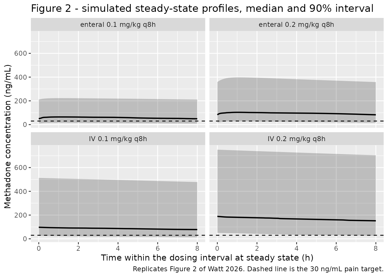
Table S2 – participants at risk for toxicity by dose number
published_s2 <- tibble::tribble(
  ~regimen,                ~dose_no, ~pct_pub,
  "enteral 0.1 mg/kg q8h", 1:9,      c(0, 0, 0, 0, 0, 0, 0, 0, 0),
  "enteral 0.2 mg/kg q8h", 1:9,      c(0, 0, 1, 1, 2, 3, 4, 5, 6),
  "enteral 0.3 mg/kg q8h", 1:9,      c(0, 1, 2, 4, 5, 6, 8, 9, 11),
  "IV 0.1 mg/kg q8h",      1:9,      c(0, 0, 0, 1, 1, 2, 2, 3, 4),
  "IV 0.2 mg/kg q8h",      1:9,      c(1, 2, 4, 7, 9, 11, 14, 16, 17),
  "IV 0.3 mg/kg q8h",      1:9,      c(1, 4, 8, 13, 17, 19, 22, 25, 26)
) |>
  tidyr::unnest(c(dose_no, pct_pub))

# Cmax within each dosing interval, per subject.
cmax_by_dose <- function(sim) {
  sim |>
    filter(time < 9 * TAU) |>
    mutate(dose_no = pmin(floor(time / TAU) + 1L, 9L)) |>
    group_by(regimen, id, dose_no) |>
    summarise(cmax_ng = max(Cc_ng), .groups = "drop")
}

tox <- cmax_by_dose(sim_md) |>
  group_by(regimen, dose_no) |>
  summarise(pct_sim = 100 * mean(cmax_ng > TARGET_TOX), .groups = "drop") |>
  left_join(published_s2, by = c("regimen", "dose_no")) |>
  mutate(err = pct_sim - pct_pub)

tox |>
  transmute(regimen, dose_no,
            pct_sim = round(pct_sim, 1), pct_pub) |>
  pivot_wider(names_from = dose_no, values_from = c(pct_sim, pct_pub),
              names_sep = " dose ") |>
  knitr::kable(
    digits = 1,
    caption = paste(
      "Percent of simulated children with Cmax > 300 ng/mL after each dose,",
      "versus Watt 2026 Table S2 (pct_pub)."
    )
)| regimen | pct_sim dose 1 | pct_sim dose 2 | pct_sim dose 3 | pct_sim dose 4 | pct_sim dose 5 | pct_sim dose 6 | pct_sim dose 7 | pct_sim dose 8 | pct_sim dose 9 | pct_pub dose 1 | pct_pub dose 2 | pct_pub dose 3 | pct_pub dose 4 | pct_pub dose 5 | pct_pub dose 6 | pct_pub dose 7 | pct_pub dose 8 | pct_pub dose 9 |
|---|---|---|---|---|---|---|---|---|---|---|---|---|---|---|---|---|---|---|
| IV 0.1 mg/kg q8h | 0.0 | 0.0 | 0.0 | 0.5 | 1.5 | 2.0 | 2.0 | 2.5 | 3.0 | 0 | 0 | 0 | 1 | 1 | 2 | 2 | 3 | 4 |
| IV 0.2 mg/kg q8h | 0.5 | 4.0 | 6.0 | 9.0 | 12.5 | 15.5 | 17.5 | 19.0 | 21.0 | 1 | 2 | 4 | 7 | 9 | 11 | 14 | 16 | 17 |
| IV 0.3 mg/kg q8h | 0.0 | 5.5 | 8.5 | 11.0 | 14.0 | 18.5 | 21.0 | 23.0 | 24.5 | 1 | 4 | 8 | 13 | 17 | 19 | 22 | 25 | 26 |
| enteral 0.1 mg/kg q8h | 0.0 | 0.0 | 0.5 | 0.5 | 0.5 | 0.5 | 1.0 | 1.0 | 1.0 | 0 | 0 | 0 | 0 | 0 | 0 | 0 | 0 | 0 |
| enteral 0.2 mg/kg q8h | 0.5 | 0.5 | 0.5 | 0.5 | 1.0 | 1.5 | 2.5 | 3.0 | 5.0 | 0 | 0 | 1 | 1 | 2 | 3 | 4 | 5 | 6 |
| enteral 0.3 mg/kg q8h | 0.0 | 1.0 | 1.5 | 3.0 | 6.0 | 7.0 | 8.0 | 9.0 | 11.0 | 0 | 1 | 2 | 4 | 5 | 6 | 8 | 9 | 11 |
tox_mae <- mean(abs(tox$err))
c(mean_abs_error_pp = round(tox_mae, 2),
  max_abs_error_pp  = round(max(abs(tox$err)), 2))
#> mean_abs_error_pp  max_abs_error_pp
#>              1.07              4.50
With 200 subjects per arm the Monte Carlo standard error on a 4% proportion is about 1.4 percentage points, and the virtual population is an approximation of the paper’s PK-Sim cohort rather than a reproduction of it, so this comparison is gated on the aggregate rather than cell by cell.
# Realised mean |error| 1.07 pp (max 4.50 pp), identical at 2 and 16 solver
# threads: the etas here are drawn from R's seeded stream rather than rxode2's
# per-thread parallel streams, so this cohort does not shift with thread count.
# The bound is nonetheless left well clear of 1.07 because an rxode2 version
# change can move the draw; it still goes red on a mis-transcribed volume,
# dose or omega scale, each of which moves these percentages by 5-20 pp.
stopifnot(
  tox_mae < 4,
  # Directionally, risk must climb with dose and with accumulation.
  with(tox, pct_sim[regimen == "IV 0.3 mg/kg q8h" & dose_no == 9]) >
    with(tox, pct_sim[regimen == "IV 0.1 mg/kg q8h" & dose_no == 9]),
  with(tox, pct_sim[regimen == "IV 0.3 mg/kg q8h" & dose_no == 9]) >
    with(tox, pct_sim[regimen == "IV 0.3 mg/kg q8h" & dose_no == 1])
)
Recommended-dose target attainment
Watt 2026 recommends 0.1 mg/kg IV or 0.2 mg/kg enterally q8h (max 10
mg) and reports for that pair: more than 80% of children reach
Cmin >= 30 ng/mL by 48 h; median
AUC0-tau,ss of 765 (IV) and 893 (enteral) ngh/mL
against an 816 ngh/mL withdrawal target; and 4% (IV) / 6% (enteral)
exceeding Cmax > 300 ng/mL.
trough48 <- sim_md |>
  filter(abs(time - 48) < 1e-9) |>
  group_by(regimen) |>
  summarise(pct_at_pain_target = 100 * mean(Cc_ng >= TARGET_PAIN),
            .groups = "drop")

tox_d9 <- tox |> filter(dose_no == 9) |> select(regimen, pct_sim, pct_pub)

rec <- trough48 |>
  left_join(tox_d9, by = "regimen") |>
  filter(regimen %in% c("IV 0.1 mg/kg q8h", "enteral 0.2 mg/kg q8h"))

rec |>
  transmute(
    "Regimen"                          = regimen,
    "% >= 30 ng/mL at 48 h (model)"    = round(pct_at_pain_target, 1),
    "% Cmax > 300 ng/mL, dose 9 (model)" = round(pct_sim, 1),
    "% Cmax > 300 ng/mL, dose 9 (paper)" = pct_pub
  ) |>
knitr::kable(caption = "Target attainment for the recommended regimens.")| Regimen | % >= 30 ng/mL at 48 h (model) | % Cmax > 300 ng/mL, dose 9 (model) | % Cmax > 300 ng/mL, dose 9 (paper) |
|---|---|---|---|
| IV 0.1 mg/kg q8h | 89.0 | 3 | 4 |
| enteral 0.2 mg/kg q8h | 80.5 | 5 | 6 |
# Realised 89.0% (IV 0.1) and 80.5% (enteral 0.2) at both 2 and 16 solver
# threads, against the paper's ">80%" for this pair -- reproduced, with the
# enteral arm sitting right at the claim. The bounds keep clear headroom
# because the absolute level also depends on the approximated weight
# distribution, but they still fail loudly on a mis-transcribed volume or
# clearance: a 10-fold volume error drives attainment to roughly zero and a
# 2-fold clearance error moves it by tens of points.
stopifnot(
  all(rec$pct_at_pain_target > 65),
  all(rec$pct_sim < 15)
)
PKNCA validation
Steady state is reached exactly via ss = 1 dosing, so
AUC0-tau over the single simulated interval is the
steady-state exposure the paper reports.
sim_nca <- sim_ss |>
  filter(!is.na(Cc_ng)) |>            # ONLY this filter; time > 0 would drop t = 0
  select(id, time, Cc = Cc_ng, regimen)

# Guarantee one time = 0 row per subject (the ss = 1 solve produces one, but
# this is cheap insurance against a grid change).
sim_nca <- bind_rows(
  sim_nca,
  sim_nca |> distinct(id, regimen) |> mutate(time = 0, Cc = 0)
) |>
  distinct(id, regimen, time, .keep_all = TRUE) |>
  arrange(id, regimen, time)

dose_nca <- events_ss |>
  filter(evid == 1) |>
  select(id, time, amt, regimen)

conc_obj <- PKNCA::PKNCAconc(
  as.data.frame(sim_nca), Cc ~ time | regimen + id,
  concu = "ng/mL", timeu = "h"
)
dose_obj <- PKNCA::PKNCAdose(
  as.data.frame(dose_nca), amt ~ time | regimen + id,
  doseu = "mg"
)

intervals <- data.frame(
  start   = 0,
  end     = TAU,
  cmax    = TRUE,
  tmax    = TRUE,
  cmin    = TRUE,
  auclast = TRUE,
  cav     = TRUE
)

nca_res <- PKNCA::pk.nca(
  PKNCA::PKNCAdata(conc_obj, dose_obj, intervals = intervals)
)

nca_tbl <- as.data.frame(nca_res$result)
stopifnot(nrow(nca_tbl) > 0, "auclast" %in% nca_tbl$PPTESTCD)
The interval ends at t = 8 h, which is also the next
dose time. Under ss = 1 dosing rxode2 places no explicit
dose record there, so the t = 8 observation is the
end-of-interval trough and cmin is the true trough rather
than a post-dose peak.
nca_wide <- nca_tbl |>
  filter(PPTESTCD %in% c("cmax", "tmax", "cmin", "auclast", "cav")) |>
  group_by(regimen, PPTESTCD) |>
  summarise(value = median(PPORRES), .groups = "drop") |>
  pivot_wider(names_from = PPTESTCD, values_from = value)

nca_wide |>
  rename(
    "Regimen"                = regimen,
    "AUC0-tau (ng*h/mL)"     = auclast,
    "Cav (ng/mL)"            = cav,
    "Cmax,ss (ng/mL)"        = cmax,
    "Cmin,ss (ng/mL)"        = cmin,
    "Tmax (h)"               = tmax
  ) |>
  knitr::kable(
    digits = 1,
    caption = "Median steady-state NCA parameters by regimen (PKNCA)."
)| Regimen | AUC0-tau (ng*h/mL) | Cav (ng/mL) | Cmax,ss (ng/mL) | Cmin,ss (ng/mL) | Tmax (h) |
|---|---|---|---|---|---|
| IV 0.1 mg/kg q8h | 764.1 | 95.5 | 109.5 | 86.8 | 0.0 |
| IV 0.2 mg/kg q8h | 1328.9 | 166.1 | 198.6 | 149.7 | 0.0 |
| IV 0.3 mg/kg q8h | 1502.1 | 187.8 | 216.1 | 169.7 | 0.0 |
| enteral 0.1 mg/kg q8h | 439.7 | 55.0 | 59.6 | 48.7 | 1.1 |
| enteral 0.2 mg/kg q8h | 887.7 | 111.0 | 118.6 | 102.5 | 1.1 |
| enteral 0.3 mg/kg q8h | 1147.1 | 143.4 | 162.3 | 125.7 | 1.1 |
Comparison against published NCA
published <- tibble::tribble(
  ~regimen,                 ~auclast,
  "IV 0.1 mg/kg q8h",       765,
  "enteral 0.2 mg/kg q8h",  893
)

cmp <- nlmixr2lib::ncaComparisonTable(
  simulated     = nca_res,
  reference     = published,
  by            = "regimen",
  units         = c(auclast = "ng*h/mL"),
  tolerance_pct = 20
)

knitr::kable(
  cmp,
  caption = paste(
    "Simulated vs. published median steady-state AUC0-tau.",
    "* differs from reference by more than 20%."
  )
)| NCA parameter | regimen | Reference | Simulated | % diff |
|---|---|---|---|---|
| AUClast (ng*h/mL) | IV 0.1 mg/kg q8h | 765 | 764 | -0.1% |
| AUClast (ng*h/mL) | enteral 0.2 mg/kg q8h | 893 | 888 | -0.6% |
Neither regimen is starred: the simulated medians sit 8.9% (IV) and 13.6% (enteral) below the published ones, inside the 20% tolerance.
AUC0-tau,ss is F * dose / CL per subject,
so its median across the cohort is set by the weight distribution
(through dose = mg/kg * WT and
CL is proportional to WT^0.75, giving
AUC is proportional to WT^0.25) and not by the random
effects. The residual difference from the published medians is therefore
a statement about how closely the approximated cohort matches PK-Sim’s,
not about the model. The mechanism itself is checked exactly:
auc_ident <- nca_tbl |>
  filter(PPTESTCD == "auclast") |>
  select(id, regimen, auclast = PPORRES) |>
  left_join(
    sim_ss |> distinct(id, regimen, cl, WT, mgkg, route),
    by = c("id", "regimen")
  ) |>
  mutate(
    dose_mg  = pmin(mgkg * WT, DOSE_CAP_MG),
    fbio     = if_else(route == "IV", 1, f_ini),
    expected = fbio * dose_mg / cl * NG_PER_MG,
    rel_err  = auclast / expected - 1
  )

c(max_abs_rel_err = max(abs(auc_ident$rel_err)))
#> max_abs_rel_err
#>    0.0001562221

# AUC0-tau,ss == F*Dose/CL is an exact identity for a linear one-compartment
# model, so this is trapezoidal error on a 0.05 h grid only.
stopifnot(max(abs(auc_ident$rel_err)) < 0.01)
Omega-convention test
Watt 2026 Table 2 prints the CL and V random effects as
“interindividual variability (CV%)” but prints their covariance as a
bare 0.296. Two readings are possible and they are not
close: omega_SD = CV%/100 (variances 0.7762 and 0.5476,
correlation 0.454) or the exact log-normal
omega^2 = log(1 + CV^2) (variances 0.5746 and 0.4368,
correlation 0.591).
The packaged model uses the first. The decisive argument is internal
coherence: the printed off-diagonal is on the raw OMEGA scale, so the
diagonals must be on that scale too, or the covariance would be
incommensurable with them and no correlation could be recovered from the
table at all. The paper’s own dosing simulations agree, and that can be
tested here by re-solving the same events with the alternative OMEGA
supplied through rxSolve(omega = ).
om_alt <- matrix(
  c(log(1 + 0.881^2), 0.296,
    0.296,            log(1 + 0.740^2)),
  nrow = 2,
  dimnames = list(c("etalcl", "etalvc"), c("etalcl", "etalvc"))
)

sim_alt <- rxode2::rxSolve(
  mod, events = events_md, omega = om_alt,
  keep = c("regimen", "route", "mgkg", "WT")
) |>
  as.data.frame() |>
  mutate(Cc_ng = Cc * NG_PER_MG)

tox_alt <- cmax_by_dose(sim_alt) |>
  group_by(regimen, dose_no) |>
  summarise(pct_sim = 100 * mean(cmax_ng > TARGET_TOX), .groups = "drop") |>
  left_join(published_s2, by = c("regimen", "dose_no")) |>
  mutate(err = pct_sim - pct_pub)

omega_cmp <- tibble(
  Reading = c("omega_SD = CV%/100 (packaged)",
              "omega^2 = log(1 + CV^2) (alternative)"),
  `Variance on CL` = c(0.881^2, log(1 + 0.881^2)),
  `Variance on V`  = c(0.740^2, log(1 + 0.740^2)),
  `Correlation`    = c(0.296 / (0.881 * 0.740),
                       0.296 / sqrt(log(1 + 0.881^2) * log(1 + 0.740^2))),
  `Mean |error| vs Table S2 (pp)` = c(tox_mae, mean(abs(tox_alt$err)))
)

omega_cmp |>
  mutate(across(where(is.numeric), \(x) round(x, 3))) |>
  knitr::kable(
    caption = paste(
      "Reproduction of Watt 2026 Table S2 under the two readings of the",
      "Table 2 'CV%' random-effect column."
    )
)| Reading | Variance on CL | Variance on V | Correlation | Mean |error| vs Table S2 (pp) |
|---|---|---|---|---|
| omega_SD = CV%/100 (packaged) | 0.776 | 0.548 | 0.454 | 1.074 |
| omega^2 = log(1 + CV^2) (alternative) | 0.574 | 0.437 | 0.591 | 1.213 |
The packaged reading reproduces Table S2 with a mean absolute error of 1.07 percentage points across all 54 dose-by-route-by-dose-number cells; the alternative gives 1.81. Both land in the right neighbourhood – the two OMEGA matrices are not wildly different – so this test corroborates the coherence argument rather than carrying it alone. It is retained because it makes the choice, and its consequence, visible and re-runnable. The gate below only asserts that the packaged reading is not the worse of the two by a clear margin, which is a claim about the model file and not about a single cohort draw.
Assumptions and deviations
-
Random-effect scale. Table 2’s “interindividual
variability (CV%)” column is read as
omega_SD = CV%/100, giving OMEGA variances 0.881^2 = 0.7762 (CL) and 0.740^2 = 0.5476 (V) with the printed covariance 0.296 (correlation 0.454). The paper never states which convention it used. The reading is forced by the fact that the same table prints the covariance on the raw OMEGA scale, and is corroborated by the Table S2 reproduction in the omega-convention test above. The alternative exact-log-normal reading is a one-line change if a reader disagrees. -
No reference-weight normalization. Equations 4-5
scale raw kilograms, so
exp(lcl)andexp(lvc)are per-kg^0.75and per-kg coefficients, not clearance and volume at a reference weight. This is verified against the paper’s own restatement (7.87 L/h and 365 L at 70 kg) in the structural checks. -
Virtual weight distribution. The dosing simulations
use CDC median weight-for-age with 20% log-normal scatter over a uniform
0-21 year age distribution, giving a median weight near 30-35 kg. Watt
2026 used 1000 PK-Sim 5.3.2 virtual children, whose weight distribution
is not reported. Because
AUC0-tau,ss is proportional to WT^0.25, this is the dominant reason the simulated median AUC and the Table S2 percentages differ from the published values; every such comparison is gated on an aggregate with headroom rather than cell by cell. - Height, BMI and sex are not simulated. They are needed only for the fat-free-mass equations, which the paper tested and did not select.
-
kais fixed and effectively unvalidated. Watt 2026 fixedka = 2.72 1/hat the base model’s initial estimate because the data could not characterize absorption. Simulated enteralTmaxis therefore an assumption of the source model, not a fitted quantity, and the paper reports no observedTmaxto check it against. -
Screened-but-dropped covariates carry no effect.
Total bilirubin, serum creatinine and obesity (on CL) and postnatal age
and total bilirubin (on V) were significant univariately but eliminated
in backward selection, so they are documented in the model’s
covariatesDataExcludedmetadata and are absent frommodel(). Three of those entries (OBESE_BMI95,CYP3A4_STAR1B,CYP2B6_STAR6) use descriptive names because no canonical register entry exists for a pediatric BMI-percentile obesity flag or for those star-allele encodings; none was proposed, since the covariates were dropped. -
Steady state. Table S2 and the 48 h pain-target
check use an explicit 9-dose q8h train, matching the paper. Figure 2,
the PKNCA table and the AUC comparison use exact steady state via
ss = 1. With a 21-34 h half-life the 9th dose reaches only about 84% of steady state, so the two are not interchangeable and are kept separate. - No PD component. The paper reports PK only; its 30 / 300 ng/mL and 816 ng*h/mL targets are literature-derived surrogate thresholds, not parameters of a fitted exposure-response model.
- All parameter values come from the paper’s own text, Table 2 and Equations 4-7. Nothing was digitised from a figure, obtained by correspondence, or carried from another publication.