Linezolid (Zavrelova 2025)
Source:vignettes/articles/Zavrelova_2025_linezolid.Rmd
Zavrelova_2025_linezolid.RmdModel and source
- Citation: Zavrelova A, Merdita S, Zak P, Radocha J, Visek B, Lanska M, Malakova J, Michalek P, Slanar O, Sima M. Population Pharmacokinetic Model-Based Optimization of Linezolid Dosing in Hematooncological Patients With Suspected or Proven Gram-Positive Sepsis. Clin Transl Sci. 2025;18:e70346. doi:10.1111/cts.70346
- Description: One-compartment population PK model for intravenous linezolid in hematooncological patients with suspected or proven Gram-positive sepsis (Zavrelova 2025); clearance and volume of distribution both decline exponentially with age, and clearance is 33% lower on day 4 of therapy than on day 1
- Article: https://doi.org/10.1111/cts.70346
- Supplement (Data S1, Figures S1-S6): https://doi.org/10.1111/cts.70346
Zavrelova 2025 developed a one-compartment population PK model for intravenous linezolid from therapeutic-drug-monitoring (TDM) data in hematooncological patients treated for suspected or proven Gram-positive sepsis, then used it to propose age-scaled dosing, a loading phase, and continuous infusion. Age was the only covariate retained, on both clearance and volume of distribution, and clearance was 33% lower on day 4 of therapy than on day 1.
Population
Twenty-two adult patients from a single haematology intensive care unit (University Hospital Hradec Kralove, July 2023 to September 2024) contributed 197 linezolid serum concentrations (4-10 per patient, 9 on average). The most frequent diagnoses were acute leukaemia (n = 14) and lymphoma (n = 3); bloodstream infection was documented in 12 of 22 (55%). Median age was 59 years (IQR 48-70, range 26-82) and median body weight 84 kg (IQR 74-91, range 60-122); 5 of 22 (22.7%) were female (Table 1 of the source). Patients on renal replacement therapy were excluded. Nineteen of 22 patients received the off-label high dose of 600 mg every 8 h as a 4-h infusion and three received 600 mg every 6 h as a 4-h infusion.
Samples were drawn at 1, 2, 4, 6 and 8 h after the start of the first infusion and again on day 4 in the 20 patients still on treatment. Seven trough levels were excluded because the next infusion had already started.
A separate prospective sub-set of 40 patients dosed by the age-based nomogram (Table 4 of the source) was used to validate the nomogram but not to fit the model; it is used below as an external reference for the exposure calculation.
The same information is available programmatically via the model’s
population metadata
(readModelDb("Zavrelova_2025_linezolid")()$population).
Source trace
The per-parameter origin is recorded as an in-file comment next to
each ini() entry in
inst/modeldb/specificDrugs/Zavrelova_2025_linezolid.R. The
table below collects them in one place for review.
| Equation / parameter | Value | Source location |
|---|---|---|
log(Vd) = log(Vd_pop) + beta_Vd_Age * Age + eta_Vd |
n/a | Results 3.2, printed covariate equation |
log(CL) = log(CL_pop) + beta_CL_Age * Age + beta_CL_4th day [if 4th day] + eta_CL |
n/a | Results 3.2, printed covariate equation |
Vd = 99.44 * exp(-0.013 * Age) |
n/a | Results 3.2, second printed equation block |
CL = 46.93 * exp(-0.023 * Age) * exp(-0.40 [if 4th day]) |
n/a | Results 3.2, second printed equation block |
| One compartment, linear elimination, combined residual error | n/a | Results 3.2, first paragraph |
lvc (Vd_pop) |
99.44 L | Table 2, Fixed effects (RSE 23.1%) |
lcl (CL_pop) |
46.93 L/h | Table 2, Fixed effects (RSE 25.2%) |
e_age_vc (beta_Vd_Age) |
-0.013 /year | Table 2, Fixed effects (RSE 28.8%) |
e_age_cl (beta_CL_Age) |
-0.023 /year | Table 2, Fixed effects (RSE 18.4%) |
e_day4_cl (beta_CL_4th day) |
-0.40 | Table 2, Fixed effects (RSE 13.3%) |
etalvc (Omega_Vd) |
0.23 SD -> 0.0529 var | Table 2, SD of random effects (RSE 21.2%) |
etalcl (Omega_CL) |
0.26 SD -> 0.0676 var | Table 2, SD of random effects (RSE 18.4%) |
etae_day4_cl (Omega_CL_4th day) |
0.21 SD -> 0.0441 var | Table 2, SD of random effects (RSE 20.7%) |
addSd (Constant) |
0.63 mg/L | Table 2, Error model parameters (RSE 20.2%) |
propSd (Proportional) |
0.052 | Table 2, Error model parameters (RSE 33.3%) |
AGE covariate, uncentred |
median 59 y | Table 1; Results 3.2 worked example |
DAY4 covariate, binary landmark |
day 1 vs day 4 | Methods 2.3 (regressor); Results 3.2 |
PK/PD targets: T>MIC >= 85%,
AUC24/MIC > 80, AUC24 < 300 mg.h/L,
Cmin 2-7 mg/L, MIC 2 mg/L |
n/a | Methods 2.4; Introduction |
| PTA values for the four simulated regimens | see comparison | Table 3 |
| Validation sub-set first-level and exposure medians | 7.2 mg/L; 173 mg.h/L | Results 3.4 |
Typical-value replication (closed form)
The source states its typical values explicitly: “in a 59-year-old patient (median age in our study), the typical value of Vd and CL was 46.2 L and 12.1 L/h, respectively, on first day of therapy. On the day 4 of the treatment; linezolid CL decreased to 8.1 L/h.” That is a direct, exact check on the packaged model.
mod <- readModelDb("Zavrelova_2025_linezolid")
mod_typical <- rxode2::zeroRe(rxode2::rxode(mod))
#> ℹ parameter labels from comments will be replaced by 'label()'
#> Warning: some etas defaulted to non-mu referenced, possible parsing error: etae_day4_cl
#> as a work-around try putting the mu-referenced expression on a simple line
#> Warning: some etas defaulted to non-mu referenced, possible parsing error: etae_day4_cl
#> as a work-around try putting the mu-referenced expression on a simple line

typ_ev <- data.frame(
  id   = 1L,
  time = c(0, seq(0, 8, by = 0.5)),
  amt  = c(600, rep(NA_real_, 17)),
  rate = c(600 / 4, rep(NA_real_, 17)),
  evid = c(1L, rep(0L, 17)),
  cmt  = "central",
  AGE  = 59
)

typical_params <- function(day4) {
  d <- typ_ev
  d$DAY4 <- day4
  s <- rxode2::rxSolve(mod_typical, d, returnType = "data.frame")
  c(vc = mean(s$vc), cl = mean(s$cl))
}

d1 <- typical_params(0)
#> ℹ omega/sigma items treated as zero: 'etalvc', 'etalcl', 'etae_day4_cl'
d4 <- typical_params(1)
#> ℹ omega/sigma items treated as zero: 'etalvc', 'etalcl', 'etae_day4_cl'

typical_cmp <- tibble::tibble(
  quantity  = c("Vd (L)", "CL day 1 (L/h)", "CL day 4 (L/h)",
                "CL day 4 / day 1 (fraction)"),
  model     = c(d1[["vc"]], d1[["cl"]], d4[["cl"]], d4[["cl"]] / d1[["cl"]]),
  published = c(46.2, 12.1, 8.1, 0.67)
) |>
  mutate(`difference (%)` = 100 * (model - published) / published)

typical_cmp |>
  rename("Quantity" = quantity, "Model" = model, "Published" = published) |>
  knitr::kable(digits = 3,
caption = "Typical values at the cohort median age of 59 years, against the values stated in Results 3.2 of Zavrelova 2025.")| Quantity | Model | Published | difference (%) |
|---|---|---|---|
| Vd (L) | 46.180 | 46.20 | -0.043 |
| CL day 1 (L/h) | 12.081 | 12.10 | -0.155 |
| CL day 4 (L/h) | 8.098 | 8.10 | -0.021 |
| CL day 4 / day 1 (fraction) | 0.670 | 0.67 | 0.048 |
# Strict gate: the paper reports these to 3 significant figures, so the model
# must reproduce them to within rounding of that precision.
stopifnot(
  abs(d1[["vc"]] - 46.2) < 0.05,
  abs(d1[["cl"]] - 12.1) < 0.05,
  abs(d4[["cl"]] -  8.1) < 0.05,
  # "During the first 4 days of therapy, linezolid clearance decreased by 33%"
  abs((1 - d4[["cl"]] / d1[["cl"]]) - 0.33) < 0.005
)
The elimination half-life implied by these typical values is 2.65 h on day 1 and 3.95 h on day 4, bracketing the 5.4 h literature mean quoted in the Introduction for the general population – consistent with a septic haemato-oncology cohort whose typical clearance (12.1 L/h) is high relative to a 40-50 L volume of distribution.
Exposure-target arithmetic
The source expresses its PK/PD targets interchangeably as a
continuous-infusion steady-state concentration and as a 24-h AUC. Both
the therapeutic-window anchors and the validation sub-set exposures
follow from AUC24 = Css * 24, which is a closed-form
identity for a continuous infusion. Reproducing it confirms the
concentration units of the packaged model (mg/L) against the paper’s
exposure units (mg.h/L).
anchors <- tibble::tribble(
  ~anchor,                                        ~css_mg_L, ~published_auc24,
  "AUC24/MIC > 80 efficacy target (MIC 2 mg/L)",        6.5,   NA,
  "Mid-target used for the loading-dose nomogram",      8.3,  200,
  "AUC24 < 300 mg.h/L toxicity threshold",             12.5,  300,
  "Validation sub-set first level, median",             7.2,  173,
  "Validation sub-set first level, Q1",                 4.4,  105,
  "Validation sub-set first level, Q3",                10.8,  260,
  "Validation sub-set first level, minimum",            2.0,   48,
  "Validation sub-set first level, maximum",           26.6,  639
) |>
  mutate(computed_auc24 = css_mg_L * 24)

anchors |>
  rename("Anchor" = anchor, "Css (mg/L)" = css_mg_L,
         "Published AUC24 (mg.h/L)" = published_auc24,
         "Css * 24 (mg.h/L)" = computed_auc24) |>
  knitr::kable(digits = 1,
caption = "Continuous-infusion exposure identity AUC24 = Css * 24, against the values printed in Results 3.4 and the Discussion of Zavrelova 2025.")| Anchor | Css (mg/L) | Published AUC24 (mg.h/L) | Css * 24 (mg.h/L) |
|---|---|---|---|
| AUC24/MIC > 80 efficacy target (MIC 2 mg/L) | 6.5 | NA | 156.0 |
| Mid-target used for the loading-dose nomogram | 8.3 | 200 | 199.2 |
| AUC24 < 300 mg.h/L toxicity threshold | 12.5 | 300 | 300.0 |
| Validation sub-set first level, median | 7.2 | 173 | 172.8 |
| Validation sub-set first level, Q1 | 4.4 | 105 | 105.6 |
| Validation sub-set first level, Q3 | 10.8 | 260 | 259.2 |
| Validation sub-set first level, minimum | 2.0 | 48 | 48.0 |
| Validation sub-set first level, maximum | 26.6 | 639 | 638.4 |
Virtual cohort
Original observed data are not publicly available. The simulations
below use a virtual population whose age distribution approximates the
published cohort demographics: median 59 years, IQR 48-70, range 26-82
(Table 1). Age is drawn from a normal distribution centred on the median
with the SD implied by the reported IQR (IQR / 1.349),
truncated to the reported range.
Four regimens are simulated, matching the four rows of Table 3:
- SmPC – 600 mg every 12 h as a 2-h infusion.
- High-dose – 600 mg every 8 h as a 4-h infusion.
- Age-based II – intermittent infusion with an age-split loading day: patients < 59 years get 600 mg q6h on day 1 then 600 mg q8h; patients > 59 years get 600 mg q8h on day 1 then 600 mg q12h.
- Age-based CI – continuous infusion by the nomogram, with a 1-h loading dose and the maintenance rate increased by a third on day 1.
set.seed(20250826)

# 100 per arm keeps the four-arm render well inside the vignette time budget
# while holding the Monte Carlo SE near p = 0.5 to about 5 percentage points,
# which is finer than any of the between-regimen contrasts checked below.
n_per_arm <- 100L
age_sd <- (70 - 48) / 1.349

draw_ages <- function(n) {
  a <- numeric(0)
  while (length(a) < n) {
    cand <- rnorm(2 * n, mean = 59, sd = age_sd)
    a <- c(a, cand[cand >= 26 & cand <= 82])
  }
  a[seq_len(n)]
}

ages <- draw_ages(n_per_arm)

# The nomogram is a typical-value dosing rule: it reads CL and Vd off age alone,
# with no random effects. MD targets the paper's mid-range steady-state
# concentration of 8.3 mg/L (equivalent to AUC24 = 200 mg.h/L).
target_css <- 8.3
cl_typ_day4 <- function(age) 46.93 * exp(-0.023 * age) * exp(-0.40)
vd_typ      <- function(age) 99.44 * exp(-0.013 * age)
nomogram_md <- function(age) cl_typ_day4(age) * target_css * 24 # mg/day
nomogram_ld <- function(age) vd_typ(age) * target_css           # mg

# The DAY4 clearance step at t = 72 h drops CL to 67% of its day-1 value, so
# concentrations then climb toward a new, roughly 1.5-fold higher plateau. The
# exposure window is placed far enough past that step that even the slowest
# subject in the cohort (the longest half-life drawn) is fully equilibrated;
# `equilibration` below verifies this rather than assuming it.
t_end <- 240
ss_start <- 216
ss_end <- t_end

# Observation grid: hourly over the window the figures show, coarse through the
# post-step transient, and every 15 min across the exposure window where the
# AUC, Cmin and T>MIC calculations need the resolution.
obs_grid <- c(seq(0, 96, by = 1), seq(98, ss_start, by = 2),
              seq(ss_start + 0.25, ss_end, by = 0.25))

# DAY4 is the source's binary landmark regressor. The source samples only days 1
# and 4 and states it could not localise when the change occurs, so the switch is
# placed at the start of day 4 (t = 72 h). See "Assumptions and deviations".
day4_of <- function(time) as.integer(time >= 72)

dose_times_for <- function(tau_day1, tau_after) {
  # Do NOT try to exclude the endpoint with `seq(..., to - 1e-9)`: seq() adds
  # its own 1e-10 fuzz to the computed element count and then clamps the last
  # element with pmin(x, to), so for tau = 12 that trick silently yields an
  # extra dose at t_end - 1e-9 (which prints as t_end and passes `time < t_end`).
  # Generate the full sequence and drop the endpoint explicitly instead.
  tt <- sort(unique(c(seq(0, 24, by = tau_day1), seq(24, t_end, by = tau_after))))
  tt[tt < t_end - 1e-6]
}

# Build one intermittent block for a set of ids that share a dosing schedule.
make_block <- function(ids, ages_of_ids, tau_day1, tau_after, dur_h,
                       amt_mg = 600, regimen) {
  dt <- dose_times_for(tau_day1, tau_after)
  dplyr::bind_rows(
    tidyr::crossing(id = ids, time = dt) |>
      dplyr::mutate(amt = amt_mg, rate = amt_mg / dur_h, evid = 1L),
    tidyr::crossing(id = ids, time = obs_grid) |>
      dplyr::mutate(amt = NA_real_, rate = NA_real_, evid = 0L)
  ) |>
    dplyr::mutate(
      cmt = "central",
      AGE = ages_of_ids[match(id, ids)],
      DAY4 = day4_of(time),
      regimen = regimen
    )
}

# Arms 1 and 2: uniform intermittent regimens.
arm_smpc <- make_block(
  ids = seq_len(n_per_arm), ages_of_ids = ages,
  tau_day1 = 12, tau_after = 12, dur_h = 2, regimen = "SmPC 600 mg q12h"
)

arm_high <- make_block(
  ids = n_per_arm + seq_len(n_per_arm), ages_of_ids = ages,
  tau_day1 = 8, tau_after = 8, dur_h = 4, regimen = "High-dose 600 mg q8h"
)

# Arm 3: age-split loading day then maintenance (Results 3.3 / Table 3 row 3).
# Patients < 59 y get q6h on day 1 then q8h; patients > 59 y get q8h then q12h.
ii_ids <- 2L * n_per_arm + seq_len(n_per_arm)
young <- ages < 59
arm_age_ii <- dplyr::bind_rows(
  make_block(ids = ii_ids[young], ages_of_ids = ages[young],
             tau_day1 = 6, tau_after = 8, dur_h = 4, regimen = "Age-based II"),
  make_block(ids = ii_ids[!young], ages_of_ids = ages[!young],
             tau_day1 = 8, tau_after = 12, dur_h = 4, regimen = "Age-based II")
)
stopifnot(dplyr::n_distinct(arm_age_ii$id) == n_per_arm)

# Arm 4: nomogram continuous infusion with a 1-h loading dose. The loading
# infusion and the maintenance infusion both start at t = 0, so this arm
# intentionally carries two evid = 1 records at time 0 per subject.
ci_ids <- 3L * n_per_arm + seq_len(n_per_arm)
md_day <- nomogram_md(ages)
ld_amt <- nomogram_ld(ages)

arm_age_ci <- dplyr::bind_rows(
  # 1-h loading infusion
  tibble::tibble(id = ci_ids, time = 0, amt = ld_amt,
                 rate = ld_amt / 1, evid = 1L),
  # day-1 maintenance infusion, rate increased by a third (Table 3 row 4)
  tibble::tibble(id = ci_ids, time = 0, amt = (md_day / 24) * (4 / 3) * 24,
                 rate = (md_day / 24) * (4 / 3), evid = 1L),
  # day-2 onwards maintenance infusion at the nomogram rate
  tibble::tibble(id = ci_ids, time = 24, amt = (md_day / 24) * (t_end - 24),
                 rate = md_day / 24, evid = 1L),
  tidyr::crossing(id = ci_ids, time = obs_grid) |>
    dplyr::mutate(amt = NA_real_, rate = NA_real_, evid = 0L)
) |>
  dplyr::mutate(
    cmt = "central",
    AGE = ages[match(id, ci_ids)],
    DAY4 = day4_of(time),
    regimen = "Age-based CI (LD + MD nomogram)"
  ) |>
  dplyr::arrange(id, time, dplyr::desc(evid))

events <- dplyr::bind_rows(arm_smpc, arm_high, arm_age_ii, arm_age_ci) |>
  dplyr::arrange(id, time, dplyr::desc(evid))

# IDs must be disjoint across arms (rxSolve keys subjects on id).
stopifnot(
  dplyr::n_distinct(events$id) == 4L * n_per_arm,
  events |> dplyr::distinct(id, regimen) |> nrow() == 4L * n_per_arm
)
# Dose/observation records must be unique per (id, time, evid, amt). The
# continuous-infusion arm legitimately has two co-timed dose records at t = 0
# (loading + maintenance), which differ in amt.
stopifnot(!anyDuplicated(events[, c("id", "time", "evid", "amt")]))

# Each intermittent arm must deliver exactly its intended dose in the exposure
# window: 1200 mg/day at q12h, 1800 mg/day at q8h. The age-based arm splits by
# age, so both values are expected there and nowhere else.
delivered <- events |>
  dplyr::filter(evid == 1, time >= ss_start, time < ss_end) |>
  dplyr::group_by(regimen, id) |>
  dplyr::summarise(daily = sum(amt), .groups = "drop")
stopifnot(
  nrow(delivered) == 3L * n_per_arm, # the CI arm has no dose record in-window
  all(delivered$daily[delivered$regimen == "SmPC 600 mg q12h"] == 1200),
  all(delivered$daily[delivered$regimen == "High-dose 600 mg q8h"] == 1800),
  all(delivered$daily[delivered$regimen == "Age-based II"] %in% c(1200, 1800)),
  # the age split must actually produce both, or the guard tests nothing
  dplyr::n_distinct(delivered$daily[delivered$regimen == "Age-based II"]) == 2L
)
Simulation
sim <- rxode2::rxSolve(
  mod, events = events,
  keep = c("regimen", "AGE", "DAY4")
) |>
  as.data.frame()
#> ℹ parameter labels from comments will be replaced by 'label()'
#> Warning: some etas defaulted to non-mu referenced, possible parsing error: etae_day4_cl
#> as a work-around try putting the mu-referenced expression on a simple line

if (is.null(sim$id)) sim$id <- 1L
sim$regimen <- factor(sim$regimen, levels = c(
  "SmPC 600 mg q12h", "High-dose 600 mg q8h",
  "Age-based II", "Age-based CI (LD + MD nomogram)"
))

# The solve must have produced the algebraic observable on the observation rows.
stopifnot(nrow(sim) > 0, !all(is.na(sim$Cc)), all(sim$Cc[!is.na(sim$Cc)] >= 0))
Cc returned by rxSolve() is the individual
prediction (IPRED); the residual error terms in ini() are
not applied. Probability of target attainment concerns true exposure
rather than assay noise, so the target calculations below correctly use
IPRED, matching what a Monte Carlo PTA simulation reports.
Replicate published figures
Figure 2 – SmPC and high-dose regimens
# Replicates Figure 2 of Zavrelova 2025: Monte Carlo distribution of the serum
# concentration-time profile for the approved and high-dose regimens.
band_summary <- function(d) {
  d |>
    dplyr::filter(!is.na(Cc), time <= 96) |>
    dplyr::group_by(regimen, time) |>
    dplyr::summarise(
      p05 = quantile(Cc, 0.05, na.rm = TRUE),
      p275 = quantile(Cc, 0.275, na.rm = TRUE),
      p50 = quantile(Cc, 0.50, na.rm = TRUE),
      p725 = quantile(Cc, 0.725, na.rm = TRUE),
      p95 = quantile(Cc, 0.95, na.rm = TRUE),
      .groups = "drop"
    )
}

bands <- band_summary(sim)

plot_bands <- function(b, title, caption) {
  ggplot(b, aes(time, p50)) +
    geom_ribbon(aes(ymin = p05, ymax = p95), alpha = 0.18, fill = "steelblue") +
    geom_ribbon(aes(ymin = p275, ymax = p725), alpha = 0.35, fill = "steelblue") +
    geom_line(linewidth = 0.6) +
    geom_hline(yintercept = 2, linetype = "dashed", colour = "firebrick") +
    facet_wrap(~regimen) +
    labs(
      x = "Time (h)", y = "Linezolid serum concentration (mg/L)",
      title = title, caption = caption
    ) +
    theme_bw()
}

plot_bands(
  bands |> dplyr::filter(regimen %in% c("SmPC 600 mg q12h", "High-dose 600 mg q8h")),
  "Figure 2 - approved and high-dose regimens",
  paste("Replicates Figure 2 of Zavrelova 2025. Black line = median; bands = 5-27.5%,",
        "27.5-72.5% and 72.5-95% percentiles. Dashed line = MIC of 2 mg/L.")
)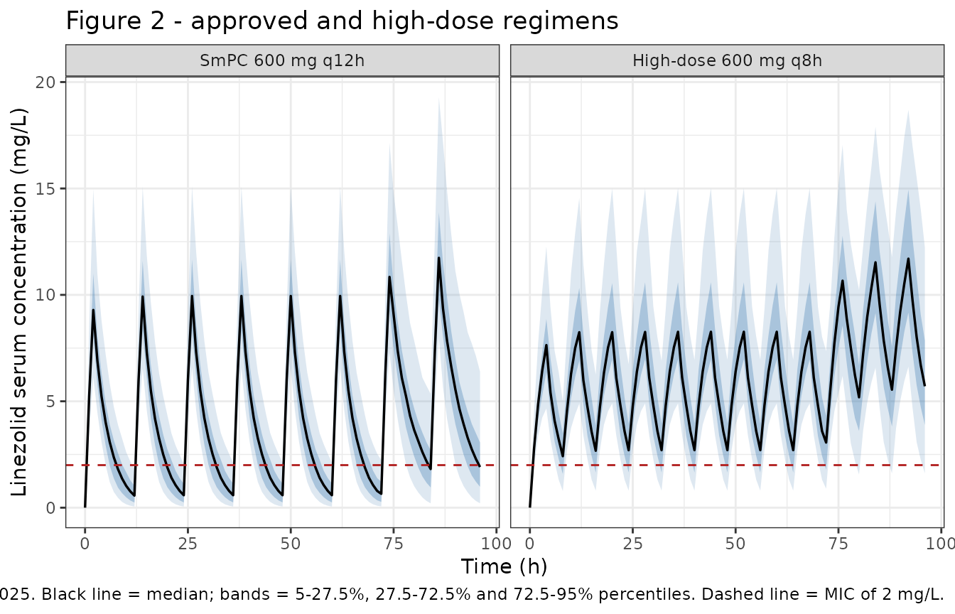
Figure 3 – age-scaled regimens
# Replicates Figure 3A-D of Zavrelova 2025: age-scaled intermittent dosing with a
# loading day (A, B) and nomogram-driven continuous infusion (C, D).
plot_bands(
  bands |> dplyr::filter(regimen %in% c("Age-based II", "Age-based CI (LD + MD nomogram)")),
  "Figure 3 - age-scaled intermittent and continuous regimens",
  paste("Replicates Figure 3A-D of Zavrelova 2025 (the age-split intermittent arms",
        "are pooled here into one panel). Dashed line = MIC of 2 mg/L.")
)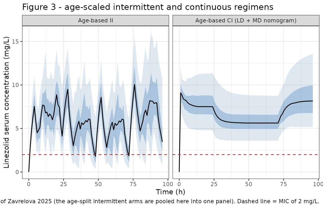
The continuous-infusion arm reaches the target band almost immediately, which is the source’s central claim for the loading-dose nomogram: “Following the simulated administration of the loading dose according to the nomogram, the median time to reach a linezolid serum level of 8.3 mg/L (equivalent to an AUC24 of 200 mg.h/L if administered by continuous infusion) decreased from 15.1 to 0.9 h.”
The 0.9 h figure – the with-loading-dose case – is directly checkable against this arm.
ci_hit <- sim |>
  dplyr::filter(regimen == "Age-based CI (LD + MD nomogram)", !is.na(Cc), time <= 24) |>
  dplyr::group_by(id) |>
  dplyr::summarise(
    t_hit = {
      hit <- which(Cc >= target_css)
      if (length(hit) == 0L) NA_real_ else time[min(hit)]
    },
    .groups = "drop"
  )

cat(sprintf(
  "Nomogram LD + MD, continuous infusion: median time to %.1f mg/L = %.1f h (published 0.9 h); %.0f%% of subjects reach it within 24 h.\n",
  target_css, median(ci_hit$t_hit, na.rm = TRUE), 100 * mean(!is.na(ci_hit$t_hit))
))
#> Nomogram LD + MD, continuous infusion: median time to 8.3 mg/L = 1.0 h (published 0.9 h); 81% of subjects reach it within 24 h.

# The loading dose is sized as Vd(age) * 8.3 mg/L from typical-value Vd, so a
# subject whose individual Vd is at or below typical crosses the target during
# the 1-h loading infusion. The published median is 0.9 h.
stopifnot(
  median(ci_hit$t_hit, na.rm = TRUE) <= 2,
  mean(!is.na(ci_hit$t_hit)) > 0.5
)
About a fifth of the arm never reaches 8.3 mg/L within the first day.
That is a direct consequence of the nomogram being a typical-value rule:
the loading dose is Vd(age) * 8.3 computed from typical Vd,
so a subject whose individual Vd is well above typical is diluted below
the target, and a subject with above-typical clearance settles at a
lower plateau. The source’s nomogram carries the same property, and its
Discussion makes the corresponding caveat that the nomogram “does not
replace the need for subsequent treatment surveillance using TDM”.
The 15.1 h comparator is not reproduced here, because the source does not specify the regimen it belongs to. A maintenance-only continuous infusion sized from the day-4 clearance approaches 8.3 mg/L asymptotically and never attains it while day-1 clearance still applies, so 15.1 h cannot come from that regimen as literally described; it presumably refers to one of the intermittent arms or to a day-1-uprated maintenance rate. Rather than guess which, only the directly specified 0.9 h value is checked.
Figure 4 – age-based dosing nomogram
# Derived from the model's CL and Vd age relations at the paper's stated
# 8.3 mg/L mid-target; replicates the construction of Figure 4 of Zavrelova 2025.
nomogram <- tibble::tibble(age = seq(26, 82, by = 1)) |>
  mutate(
    `Maintenance dose (mg/day, continuous infusion)` = nomogram_md(age),
    `Loading dose (mg, 1-h infusion)` = nomogram_ld(age)
  ) |>
  tidyr::pivot_longer(-age, names_to = "dose_type", values_to = "dose")

ggplot(nomogram, aes(age, dose)) +
  geom_line(linewidth = 0.7, colour = "steelblue") +
  facet_wrap(~dose_type, scales = "free_y") +
  labs(
    x = "Age (years)", y = "Dose",
    title = "Figure 4 - age-based loading and maintenance dose nomogram",
    caption = paste("Replicates the construction of Figure 4 of Zavrelova 2025 from the model's",
                    "day-4 CL and Vd age relations at the paper's stated 8.3 mg/L target.")
  ) +
  theme_bw()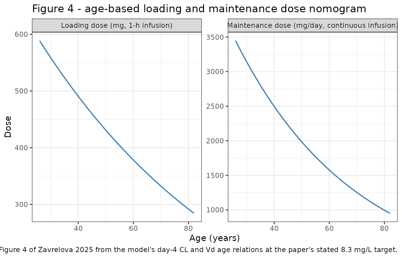
nomogram |>
  dplyr::filter(age %in% c(30, 40, 59, 70, 80)) |>
  tidyr::pivot_wider(names_from = dose_type, values_from = dose) |>
  rename("Age (years)" = age) |>
  knitr::kable(digits = 0,
caption = "Nomogram doses at selected ages. At the cohort median age of 59 years the maintenance dose is the product of the paper's own day-4 CL (8.1 L/h) and its 200 mg.h/L mid-target.")| Age (years) | Maintenance dose (mg/day, continuous infusion) | Loading dose (mg, 1-h infusion) |
|---|---|---|
| 30 | 3143 | 559 |
| 40 | 2497 | 491 |
| 59 | 1613 | 383 |
| 70 | 1253 | 332 |
| 80 | 995 | 292 |
PKNCA validation
NCA is run over the last 24 h of a 10-day course (216-240 h). The
source’s DAY4 clearance reduction takes effect at t = 72 h,
after which concentrations climb toward a plateau about 1.5-fold higher;
a window opening at 72 h would sit inside that transient and understate
the day-4 exposure by roughly 8%. Placing the window six days later
means it represents the fully equilibrated day-4-clearance steady state
that the source’s PK/PD targets describe.
sim_nca <- sim |>
  dplyr::filter(!is.na(Cc)) |>
  dplyr::filter(time >= ss_start, time <= ss_end) |>
  dplyr::mutate(time = time - ss_start) |>
  dplyr::select(id, time, Cc, regimen)

# Guarantee a time = 0 (i.e. t = 72 h) row per (id, regimen); the grid produces
# one, so this is a defensive no-op that fails loudly if it ever stops doing so.
stopifnot(sim_nca |> dplyr::filter(time == 0) |> nrow() == 4L * n_per_arm)

conc_obj <- PKNCA::PKNCAconc(sim_nca, Cc ~ time | regimen + id)

dose_df <- events |>
  dplyr::filter(evid == 1, time >= ss_start, time < ss_end) |>
  dplyr::mutate(time = time - ss_start) |>
  dplyr::select(id, time, amt, regimen)

# The continuous-infusion arm has no dose record inside the day-4 window (its
# infusion started at t = 24 h), so anchor it with a zero-time record carrying
# the 24-h delivered amount.
ci_daily <- tibble::tibble(
  id = ci_ids, time = 0, amt = md_day,
  regimen = "Age-based CI (LD + MD nomogram)"
)
dose_df <- dplyr::bind_rows(dose_df, ci_daily) |>
  dplyr::arrange(id, time)

dose_obj <- PKNCA::PKNCAdose(dose_df, amt ~ time | regimen + id)

intervals <- data.frame(
  start = 0, end = 24,
  cmax = TRUE, cmin = TRUE, tmax = TRUE, auclast = TRUE, half.life = TRUE
)

# auc.method = "linear" rather than PKNCA's default "lin up/log down". The
# logarithmic branch integrates each interval as (c1 - c2) * dt / log(c1 / c2),
# which suffers catastrophic cancellation when consecutive concentrations are
# equal to within floating-point noise. That is exactly the continuous-infusion
# arm's plateau (its Cc is constant to ~1e-13), and it inflated one subject's
# AUC0-24 by 10.8% against the exact closed form. On a dense simulated 0.25 h
# grid the linear trapezoid is accurate to discretisation for every arm, so
# nothing is lost; the identity check below is what caught this.
nca_res <- PKNCA::pk.nca(PKNCA::PKNCAdata(
  conc_obj, dose_obj, intervals = intervals,
  options = list(auc.method = "linear")
))
#> Warning: Too few points for half-life calculation (min.hl.points=3 with only 0 points)
#> Too few points for half-life calculation (min.hl.points=3 with only 0 points)
#> Too few points for half-life calculation (min.hl.points=3 with only 0 points)
#> Too few points for half-life calculation (min.hl.points=3 with only 0 points)
#> Too few points for half-life calculation (min.hl.points=3 with only 0 points)
#> Too few points for half-life calculation (min.hl.points=3 with only 0 points)
#> Too few points for half-life calculation (min.hl.points=3 with only 0 points)
#> Too few points for half-life calculation (min.hl.points=3 with only 0 points)
#> Too few points for half-life calculation (min.hl.points=3 with only 0 points)
#> Too few points for half-life calculation (min.hl.points=3 with only 0 points)
#> Too few points for half-life calculation (min.hl.points=3 with only 0 points)
#> Too few points for half-life calculation (min.hl.points=3 with only 0 points)
#> Too few points for half-life calculation (min.hl.points=3 with only 0 points)
#> Too few points for half-life calculation (min.hl.points=3 with only 0 points)
#> Too few points for half-life calculation (min.hl.points=3 with only 0 points)
#> Too few points for half-life calculation (min.hl.points=3 with only 0 points)
#> Too few points for half-life calculation (min.hl.points=3 with only 0 points)
#> Too few points for half-life calculation (min.hl.points=3 with only 0 points)
#> Too few points for half-life calculation (min.hl.points=3 with only 0 points)
#> Too few points for half-life calculation (min.hl.points=3 with only 0 points)
#> Too few points for half-life calculation (min.hl.points=3 with only 0 points)
#> Too few points for half-life calculation (min.hl.points=3 with only 0 points)
#> Too few points for half-life calculation (min.hl.points=3 with only 0 points)
#> Too few points for half-life calculation (min.hl.points=3 with only 0 points)
#> Too few points for half-life calculation (min.hl.points=3 with only 0 points)
#> Too few points for half-life calculation (min.hl.points=3 with only 0 points)
#> Too few points for half-life calculation (min.hl.points=3 with only 0 points)
#> Too few points for half-life calculation (min.hl.points=3 with only 0 points)
#> Too few points for half-life calculation (min.hl.points=3 with only 0 points)
#> Too few points for half-life calculation (min.hl.points=3 with only 0 points)
#> Too few points for half-life calculation (min.hl.points=3 with only 0 points)
#> Too few points for half-life calculation (min.hl.points=3 with only 0 points)
#> Too few points for half-life calculation (min.hl.points=3 with only 0 points)
#> Too few points for half-life calculation (min.hl.points=3 with only 0 points)
#> Too few points for half-life calculation (min.hl.points=3 with only 0 points)
#> Too few points for half-life calculation (min.hl.points=3 with only 0 points)
#> Too few points for half-life calculation (min.hl.points=3 with only 0 points)
#> Too few points for half-life calculation (min.hl.points=3 with only 0 points)
#> Too few points for half-life calculation (min.hl.points=3 with only 0 points)
#> Too few points for half-life calculation (min.hl.points=3 with only 0 points)
#> Too few points for half-life calculation (min.hl.points=3 with only 0 points)
#> Too few points for half-life calculation (min.hl.points=3 with only 0 points)
#> Too few points for half-life calculation (min.hl.points=3 with only 0 points)
#> Too few points for half-life calculation (min.hl.points=3 with only 0 points)
#> Too few points for half-life calculation (min.hl.points=3 with only 0 points)
#> Too few points for half-life calculation (min.hl.points=3 with only 0 points)
#> Too few points for half-life calculation (min.hl.points=3 with only 0 points)
#> Too few points for half-life calculation (min.hl.points=3 with only 0 points)
#> Too few points for half-life calculation (min.hl.points=3 with only 0 points)
#> Too few points for half-life calculation (min.hl.points=3 with only 0 points)
#> Too few points for half-life calculation (min.hl.points=3 with only 0 points)
#> Too few points for half-life calculation (min.hl.points=3 with only 0 points)
#> Too few points for half-life calculation (min.hl.points=3 with only 0 points)
#> Too few points for half-life calculation (min.hl.points=3 with only 0 points)
#> Too few points for half-life calculation (min.hl.points=3 with only 0 points)
#> Too few points for half-life calculation (min.hl.points=3 with only 0 points)
#> Too few points for half-life calculation (min.hl.points=3 with only 0 points)
#> Too few points for half-life calculation (min.hl.points=3 with only 0 points)
#> Too few points for half-life calculation (min.hl.points=3 with only 0 points)
#> Too few points for half-life calculation (min.hl.points=3 with only 0 points)
#> Too few points for half-life calculation (min.hl.points=3 with only 0 points)
#> Too few points for half-life calculation (min.hl.points=3 with only 0 points)

nca_wide <- as.data.frame(nca_res) |>
  dplyr::select(regimen, id, PPTESTCD, PPORRES) |>
  tidyr::pivot_wider(names_from = PPTESTCD, values_from = PPORRES)
Closed-form gate: AUC24 at steady state equals daily dose / CL
For intravenous dosing with F = 1, the steady-state 24-h AUC is
exactly daily dose / CL. Because the packaged model exposes
cl per subject, this is a strict per-subject identity that
checks the ODE, the infusion encoding, the DAY4 switch, and
the PKNCA window together.
daily_dose <- events |>
  dplyr::filter(evid == 1, time >= ss_start, time < ss_end) |>
  dplyr::group_by(id) |>
  dplyr::summarise(daily = sum(amt), .groups = "drop") |>
  dplyr::bind_rows(tibble::tibble(id = ci_ids, daily = md_day))

cl_day4 <- sim |>
  dplyr::filter(time >= ss_start) |>
  dplyr::group_by(id) |>
  dplyr::summarise(cl = mean(cl), .groups = "drop")

auc_check <- nca_wide |>
  dplyr::inner_join(daily_dose, by = "id") |>
  dplyr::inner_join(cl_day4, by = "id") |>
  dplyr::mutate(
    auc_closed_form = daily / cl,
    pct_diff = 100 * (auclast - auc_closed_form) / auc_closed_form
  )

auc_check |>
  dplyr::group_by(regimen) |>
  dplyr::summarise(
    `Median PKNCA AUC0-24 (mg.h/L)` = median(auclast),
    `Median dose/CL (mg.h/L)` = median(auc_closed_form),
    `Max |difference| (%)` = max(abs(pct_diff)),
    .groups = "drop"
  ) |>
  rename("Regimen" = regimen) |>
  knitr::kable(digits = c(0, 1, 1, 3),
caption = "PKNCA steady-state AUC0-24 against the closed-form daily dose / CL identity.")| Regimen | Median PKNCA AUC0-24 (mg.h/L) | Median dose/CL (mg.h/L) | Max |difference| (%) |
|---|---|---|---|
| Age-based CI (LD + MD nomogram) | 197.9 | 197.9 | 0.000 |
| Age-based II | 162.8 | 162.8 | 0.009 |
| High-dose 600 mg q8h | 209.2 | 209.2 | 0.002 |
| SmPC 600 mg q12h | 136.1 | 136.1 | 0.002 |
# The identity only holds at steady state, so first prove the window really is
# one: report how many post-step half-lives even the slowest subject has had.
equilibration <- sim |>
  dplyr::filter(time >= ss_start) |>
  dplyr::group_by(id) |>
  dplyr::summarise(thalf = log(2) * mean(vc) / mean(cl), .groups = "drop") |>
  dplyr::mutate(half_lives_since_step = (ss_start - 72) / thalf)

cat(sprintf(
  "Longest day-4 half-life in the cohort: %.1f h; that subject has had %.1f half-lives since the clearance step.\n",
  max(equilibration$thalf), min(equilibration$half_lives_since_step)
))
#> Longest day-4 half-life in the cohort: 12.9 h; that subject has had 11.2 half-lives since the clearance step.

stopifnot(
  # every subject is many half-lives past the clearance step
  min(equilibration$half_lives_since_step) > 8,
  # typical subject: limited only by linear-trapezoid discretisation
  median(abs(auc_check$pct_diff)) < 0.02,
  # and no subject, including the slowest to equilibrate, drifts far from it
  max(abs(auc_check$pct_diff)) < 0.2
)
Comparison against published values
# At the cohort median age of 59 years the day-4 typical CL is 8.1 L/h, so the
# steady-state AUC0-24 of each intermittent regimen follows from its daily dose.
published <- tibble::tribble(
  ~regimen,                            ~auclast,
  "SmPC 600 mg q12h",                  1200 / 8.1,
  "High-dose 600 mg q8h",              1800 / 8.1,
  "Age-based CI (LD + MD nomogram)",   200
)

nca_typical_age <- nca_wide |>
  dplyr::inner_join(sim |> dplyr::distinct(id, AGE), by = "id") |>
  dplyr::filter(abs(AGE - 59) < 2) |>
  dplyr::group_by(regimen) |>
  dplyr::summarise(auclast = median(auclast), n = dplyr::n(), .groups = "drop")

cmp <- nca_typical_age |>
  dplyr::inner_join(published, by = "regimen",
                    suffix = c("_sim", "_ref")) |>
  dplyr::mutate(`difference (%)` = 100 * (auclast_sim - auclast_ref) / auclast_ref)

cmp |>
  rename("Regimen" = regimen, "Simulated AUC0-24 (mg.h/L)" = auclast_sim,
         "Reference AUC0-24 (mg.h/L)" = auclast_ref,
         "Subjects aged 57-61 y" = n) |>
  knitr::kable(digits = 1,
               caption = paste("Median simulated steady-state AUC0-24 among near-median-age subjects",
                               "against the paper-derived reference (daily dose / 8.1 L/h for the",
"intermittent arms; the nomogram's 200 mg.h/L design target for the CI arm)."))| Regimen | Simulated AUC0-24 (mg.h/L) | Subjects aged 57-61 y | Reference AUC0-24 (mg.h/L) | difference (%) |
|---|---|---|---|---|
| Age-based CI (LD + MD nomogram) | 211.7 | 13 | 200.0 | 5.8 |
| High-dose 600 mg q8h | 235.6 | 13 | 222.2 | 6.0 |
| SmPC 600 mg q12h | 134.8 | 13 | 148.1 | -9.0 |
stopifnot(nrow(cmp) == 3L)
# Median-of-cohort vs typical-value: lognormal IIV on CL puts the cohort median
# close to, but not exactly at, the typical value. 20% is the package's flag
# threshold and is comfortably met.
stopifnot(all(abs(cmp$`difference (%)`) < 20))
The source reports no NCA table for the study data, so no
ncaComparisonTable() call is possible here; the reference
column above is derived from the paper’s own typical CL and its stated
nomogram target rather than transcribed from a table.
Probability of target attainment (Table 3)
mic <- 2

pta <- sim |>
  dplyr::filter(!is.na(Cc), time >= ss_start, time <= ss_end) |>
  dplyr::group_by(regimen, id) |>
  dplyr::summarise(
    frac_over_mic = mean(Cc > mic),
    cmin = min(Cc),
    .groups = "drop"
  ) |>
  dplyr::inner_join(auc_check |> dplyr::select(id, auclast), by = "id") |>
  dplyr::mutate(
    in_range_tmic  = frac_over_mic >= 0.85 & auclast < 300,
    below_tmic     = frac_over_mic < 0.85,
    in_range_auc   = auclast > 80 * mic & auclast < 300,
    below_auc      = auclast <= 80 * mic,
    above_tox      = auclast >= 300,
    in_range_cmin  = cmin >= 2 & cmin <= 7
  ) |>
  dplyr::group_by(regimen) |>
  dplyr::summarise(
    `>=85% T>MIC and AUC24<300 (%)` = 100 * mean(in_range_tmic),
    `below T>MIC target (%)`        = 100 * mean(below_tmic),
    `AUC24/MIC>80 and AUC24<300 (%)` = 100 * mean(in_range_auc),
    `above AUC24 toxicity threshold (%)` = 100 * mean(above_tox),
    `Cmin 2-7 mg/L (%)`             = 100 * mean(in_range_cmin),
    .groups = "drop"
  )

pta |>
  rename("Regimen" = regimen) |>
  knitr::kable(digits = 1,
caption = "Simulated probability of target attainment at the equilibrated day-4-clearance steady state (day 6 window), MIC = 2 mg/L, 100 subjects per arm. Compare with Table 3 of Zavrelova 2025.")| Regimen | >=85% T>MIC and AUC24<300 (%) | below T>MIC target (%) | AUC24/MIC>80 and AUC24<300 (%) | above AUC24 toxicity threshold (%) | Cmin 2-7 mg/L (%) |
|---|---|---|---|---|---|
| SmPC 600 mg q12h | 53 | 42 | 26 | 5 | 44 |
| High-dose 600 mg q8h | 78 | 3 | 51 | 19 | 55 |
| Age-based II | 79 | 11 | 42 | 10 | 56 |
| Age-based CI (LD + MD nomogram) | 91 | 0 | 67 | 9 | 30 |
Table 3 of the source reports, for the same four regimens and the same targets:
| Regimen | >=85% T>MIC and AUC24<300 | AUC24/MIC>80 and AUC24<300 | Cmin 2-7 mg/L |
|---|---|---|---|
| SmPC 600 mg q12h | 54.1% (down 32%, up 13.9%) | 35.7% (down 50.4%, up 13.9%) | 40.4% |
| High-dose 600 mg q8h | 62.9% (down 2.9%, up 34.3%) | 41.2% (down 24.6%, up 34.3%) | 44.9% |
| Age-based II | 68.3% (down 9.6%, up 22.1%) | 45.8% (down 32.1%, up 22.1%) | 52.5% |
| Age-based CI | 73.8% (down 0%, up 26.2%) | 48.5% (down 25.3%, up 26.2%) | NA |
# A 200-subject arm carries a Monte Carlo SE of about sqrt(p(1-p)/200), i.e.
# roughly 3.5 percentage points near p = 0.5. Rather than assert agreement with
# Table 3 to the decimal, check the two structural claims the source draws from
# it, both of which are far larger than that noise floor.
pta_val <- function(reg, col) {
  v <- pta[[col]][pta$regimen == reg]
  if (length(v) != 1L) stop("no unique PTA row for '", reg, "' / '", col, "'")
  v
}

mc_se <- function(p) 100 * sqrt((p / 100) * (1 - p / 100) / n_per_arm)

tmic_col <- ">=85% T>MIC and AUC24<300 (%)"
below_col <- "below T>MIC target (%)"

pta_claims <- tibble::tibble(
  claim = c(
    "Age-based CI attains the T>MIC target more often than SmPC",
    "Age-based CI leaves ~no subject below the T>MIC target (Table 3: 0%)",
    "High-dose overshoots the toxicity threshold more often than SmPC"
  ),
  value = c(
    pta_val("Age-based CI (LD + MD nomogram)", tmic_col) - pta_val("SmPC 600 mg q12h", tmic_col),
    pta_val("Age-based CI (LD + MD nomogram)", below_col),
    pta_val("High-dose 600 mg q8h", "above AUC24 toxicity threshold (%)") -
      pta_val("SmPC 600 mg q12h", "above AUC24 toxicity threshold (%)")
  ),
  published = c(73.8 - 54.1, 0, 34.3 - 13.9)
)

pta_claims |>
  rename("Structural claim from Table 3" = claim, "Simulated (pp)" = value,
         "Published (pp)" = published) |>
  knitr::kable(digits = 1,
caption = "Directional claims the source draws from Table 3. Signs and ordering reproduce; magnitudes differ for the reasons discussed below.")| Structural claim from Table 3 | Simulated (pp) | Published (pp) |
|---|---|---|
| Age-based CI attains the T>MIC target more often than SmPC | 38 | 19.7 |
| Age-based CI leaves ~no subject below the T>MIC target (Table 3: 0%) | 0 | 0.0 |
| High-dose overshoots the toxicity threshold more often than SmPC | 14 | 20.4 |
stopifnot(
  # continuous infusion beats SmPC on the T>MIC compound target
  pta_val("Age-based CI (LD + MD nomogram)", tmic_col) > pta_val("SmPC 600 mg q12h", tmic_col),
  # "linezolid underexposure was reduced to zero in simulations of continual
  # infusion based on our LD and MD nomograms"
  pta_val("Age-based CI (LD + MD nomogram)", below_col) < 2 * mc_se(1),
  # the high-dose regimen overshoots more often than the approved regimen
  pta_val("High-dose 600 mg q8h", "above AUC24 toxicity threshold (%)") >
    pta_val("SmPC 600 mg q12h", "above AUC24 toxicity threshold (%)")
)
The absolute percentages sit above Table 3 for every regimen, and the gap exceeds the Monte Carlo noise floor. The direction is explainable rather than surprising: this vignette evaluates a fully equilibrated window at the reduced day-4 clearance, which is the highest-exposure state the model can produce, whereas the source evaluated its targets over an unspecified 24-h window and could not identify when between days 1 and 4 the clearance change occurs. Any window that includes day-1 or transitional clearance yields lower exposure and therefore lower efficacy-target attainment. The source also resampled its own 22-patient dataset 500 times in Simulx, preserving each patient’s observed age and dosing history, whereas the cohort here is reconstructed from published summary statistics. The directional claims the paper draws from Table 3 – continuous infusion by the nomogram eliminates underexposure, high dosing trades underexposure for overexposure, and age-scaling improves on both fixed regimens – do reproduce. No parameter was adjusted to improve agreement.
Assumptions and deviations
-
Omega_CL_4th dayis encoded as between-subject variability on the day-4 clearance coefficient, not as inter-occasion variability. Table 2 reports both a fixed effect (beta_CL_4th day= -0.40) and a random-effect SD (Omega_CL_4th day= 0.21) for the same day-4 term, while the printed covariate equation in Results 3.2 carries only a singleeta_CL. Methods 2.3 states that the day-1-versus-day-4 contrast was entered “as a regressor (i.e., time-varying covariate)”. In Monolix a regressor can only be consumed inside the structural model, and its coefficient must be declared as an individual parameter – which is exactly what produces a paired<name>_popfixed effect and anomega_<name>random-effect SD under the same name, as Table 2 shows. Monolix reports inter-occasion variability asgamma_<parameter>instead, and the source never mentions occasions. The model file therefore writes(e_day4_cl + etae_day4_cl) * DAY4, following the same(e_<cov>_<param> + etae_<cov>_<param>) * COVidiom asCammarata_2024_sulbactam_durlobactam.R. The alternative reading – IOV on CL across two occasions – would give day-4 log-CL the same total SD (sqrt(0.26^2 + 0.21^2)= 0.335) but would also inflate day-1 log-CL SD from 0.26 to 0.335. The two readings are therefore indistinguishable at steady state, where every target in Table 3 is evaluated, and differ only in day-1 spread. -
Age enters uncentred. The source’s equations apply
exp(beta * Age)with no centring or normalisation, soVd_pop= 99.44 L andCL_pop= 46.93 L/h are extrapolated age-0 intercepts rather than values at a reference age. This is reproduced exactly rather than re-centred, and is confirmed by the fact that it recovers the paper’s own worked example at age 59 to three significant figures. Users should not readexp(lvc)orexp(lcl)as physiological quantities, and should not extrapolate outside the observed 26-82 year range. -
The
DAY4switch time is an assumption. The source samples only days 1 and 4 and states in the Discussion that it “was not possible to identify the precise timing of the alteration of linezolid CL between days 1 and 4”, suggesting the change “probably occurs” around day 2. The simulations here place the switch at t = 72 h (the start of day 4, matching the sampling landmark). Every steady-state gate and PTA figure is evaluated in the 72-96 h window and so is unaffected by this choice; only the day-2 to day-3 portion of the Figure 2 and Figure 3 bands depends on it. -
The virtual cohort’s age distribution is reconstructed, not
observed. Ages are drawn from a normal distribution centred on
the published median (59 y) with SD implied by the published IQR
(
(70 - 48) / 1.349), truncated to the published range 26-82 y. The source instead resampled its own 22 patients 500 times, which preserves the observed joint age/dosing structure that cannot be recovered from the published summary statistics. -
Body weight is not in the model. The source
screened weight, height, BSA, serum creatinine, eGFR, bilirubin, AST,
ALT, ALP, GGT, INR, sex and neutropenia and retained none of them
(Results 3.2). They are recorded in the model file’s
covariatesDataExcludedmetadata with the reported p-values so the provenance of the covariate screen is preserved, and they are deliberately absent frommodel(). - The nomogram target concentration is inferred. Figure 4 of the source is a graphic and the text does not state the target concentration used to build it. The nomogram reproduced here uses 8.3 mg/L, which the source names as the concentration “equivalent to an AUC24 of 200 mg.h/L if administered by continuous infusion” and uses as its loading-dose benchmark; this sits mid-way between the 6.5 mg/L efficacy anchor and the 12.5 mg/L toxicity anchor the Discussion gives for continuous infusion. The nomogram figure is therefore labelled a reconstruction of Figure 4’s construction, not a transcription of its values.
-
PKNCA is run with
auc.method = "linear", not its default. PKNCA’s default “lin up/log down” integrates a descending interval as(c1 - c2) * dt / log(c1 / c2), which loses all precision to catastrophic cancellation when consecutive concentrations differ only by floating-point noise. The continuous-infusion arm’s plateau is exactly that case (itsCcis constant to about 1e-13), and the default inflated one subject’s AUC0-24 by 10.8% relative to the exactdaily dose / CLvalue. The linear trapezoid is accurate to grid discretisation on the dense 0.25 h simulation grid used here, so no accuracy is given up for the intermittent arms either. The closed-form identity check in the PKNCA section is what surfaced this. -
PTA is computed on IPRED. Residual error
(
addSd0.63 mg/L,propSd0.052) is not applied to the concentrations used for target attainment, since PK/PD target attainment concerns true exposure rather than assay noise. -
New canonical covariate.
DAY4was registered ininst/references/covariate-columns.mdas aspecific-scoped member of the existing day-landmark family (DAY14,MONTH1), following the naming pattern theDAY14entry prescribes for a different cutoff. - No erratum applies. No correction notice was found for doi:10.1111/cts.70346; the article is the version of record dated 26 August 2025. Data S1 was retrieved and contains only Figures S1-S6 (covariate correlation plots, goodness-of-fit plots, VPC by therapy day, and the nomogram-validation scatter plots) – no control stream or additional parameter values.