Doxycycline + florfenicol against Riemerella anatipestifer in ducks (Li 2025)
Source:vignettes/articles/Li_2025_doxycycline_florfenicol_ducks.Rmd
Li_2025_doxycycline_florfenicol_ducks.RmdModel and source
- Citation: Li FL, He CY, Chen HY, Cheng SM, Liu Y, Ding HZ, Zhang HL. (2025). In vivo pharmacokinetic/pharmacodynamic relationship of florfenicol in combination with doxycycline against Riemerella anatipestifer in ducks and the effect upon resistance development. Poultry Science 104:104922. doi:10.1016/j.psj.2025.104922.
- Article: https://doi.org/10.1016/j.psj.2025.104922
Li 2025 studied doxycycline (DOX) given as a single intramuscular injection to Riemerella anatipestifer-infected ducks, and related its exposure to the 24 h change in bacterial count when it was combined with a fixed background dose of florfenicol (FF). The only drug with a pharmacokinetic model in this paper is doxycycline; florfenicol enters solely as the 20 or 40 mg/kg background arm that stratifies the exposure-response fit, and its own half-life is quoted from the authors’ earlier work rather than modelled here.
The paper contains four independent WinNonlin fits, so the extraction is four model files, all pointing at this one vignette:
| Model | What it is | Source |
|---|---|---|
Li_2025_doxycycline_duck_ff20 |
Plasma PK + exposure-response, FF 20 mg/kg background | Table 1 (plasma), Table 2 |
Li_2025_doxycycline_duck_ff40 |
Plasma PK + exposure-response, FF 40 mg/kg background | Table 1 (plasma), Table 3 |
Li_2025_doxycycline_duck_lung |
Lung tissue PK | Table 1 (lung) |
Li_2025_doxycycline_duck_liver |
Liver tissue PK | Table 1 (liver) |
ff20 <- readModelDb("Li_2025_doxycycline_duck_ff20")
ff40 <- readModelDb("Li_2025_doxycycline_duck_ff40")
lung <- readModelDb("Li_2025_doxycycline_duck_lung")
liver <- readModelDb("Li_2025_doxycycline_duck_liver")
Population
Seven-day-old common shelducks (Tadorna tadorna) weighing 130-150 g, obtained from a commercial farm in Guangxi, China. Systemic infection was established by intraperitoneal injection of R. anatipestifer at 109 CFU/mL; the target bacterial load was reached 12 h after inoculation, at which point drug was given.
The PK cohort was five groups of 72 ducks receiving DOX at 1, 2.5, 5, 10 and 20 mg/kg intramuscularly into the thigh, with plasma, lung and liver sampled at 0.5, 1, 2, 4, 6, 8, 12, 24 and 36 h. The single-dose PD study used 15 groups of eight ducks (10 FF + DOX combinations, four monotherapy arms, one untreated model group). A further nine groups of eight ducks received two doses in 24 h against the less susceptible RA38 strain; no exposure-response model was fitted to that experiment.
The challenge strain for the modelled experiments was R.
anatipestifer CVCC3857, with a doxycycline MIC of 1 ug/mL and a
florfenicol MIC of 1 ug/mL (Results, “MIC and MPC Of FF and DOX against
RA”). Doxycycline plasma protein binding was measured by equilibrium
dialysis at 0.1, 1 and 10 ug/mL as 37.84%, 29.92% and 44.33% (mean
37.36%), giving fu = 0.6264.
The same information is available programmatically via
rxode2::rxode(readModelDb("Li_2025_doxycycline_duck_ff20"))$population.
Source trace
Every packaged value with its location in Li 2025. Entries marked derived are computed from tabulated values by the identity shown; the derivations are validated numerically in the next section.
| Equation / parameter | Value | Source location |
|---|---|---|
| One-compartment first-order-absorption PK equation | n/a | Methods, “Pharmacokinetics (PK) of DOX in RA-infected ducks” |
| Inhibitory sigmoid Emax equation | n/a | Methods, “PK and PD analyses” |
| Toutain dose equation | n/a | Methods, “Dose calculations” |
lka (plasma) |
log(log(2)/0.60) |
Table 1, plasma mean T1/2ka = 0.60 +/- 0.20 h |
lcl (plasma) |
log(0.40) |
Table 1, plasma mean Cl/F = 0.40 +/- 0.08 L/h/kg |
lvc (plasma) |
log(0.40/(log(2)/11.21)) |
derived V/F = (Cl/F)/kel; Table 1 plasma mean T1/2kel = 11.21 +/- 0.99 h |
fu |
1 - 0.3736 |
Results, “PK of DOX in ducks”; Methods, “Dose calculations” (62.64%) |
mic |
1 |
Results, “MIC and MPC Of FF and DOX against RA”; Table 4, row
3857(original)
|
e0 (FF 20) |
-0.53 |
Table 2, row “E max” = 0.53, sign flipped (see Errata) |
lemax (FF 20) |
log(3.98) |
Table 2, row “E 0” = 3.98 |
lec50 (FF 20) |
log(8.83) |
Table 2, row “EC 50”, AUC24h/MIC column |
lhill (FF 20) |
log(0.86) |
Table 2, row “Hill’s slope”, AUC24h/MIC column |
e0 (FF 40) |
-0.06 |
Table 3, row “E max” = 0.06, sign flipped |
lemax (FF 40) |
log(4.76) |
Table 3, row “E 0” = 4.76 (see Errata) |
lec50 (FF 40) |
log(16.97) |
Table 3, row “EC 50”, AUC24h/MIC column |
lhill (FF 40) |
log(0.63) |
Table 3, row “Hill’s slope”, AUC24h/MIC column |
lka (lung) |
log(log(2)/0.42) |
Table 1, lung mean T1/2ka = 0.42 +/- 0.14 h |
lcl (lung) |
log(0.3287) |
derived mean of dose/AUC over the five dose levels |
lvc (lung) |
log(0.3287/(log(2)/11.53)) |
derived; Table 1 lung mean T1/2kel = 11.53 +/- 1.43 h |
lka (liver) |
log(log(2)/0.47) |
Table 1, liver mean T1/2ka = 0.47 +/- 0.13 h |
lcl (liver) |
log(0.1350) |
derived mean of dose/AUC over the five dose levels |
lvc (liver) |
log(0.1350/(log(2)/13.01)) |
derived; Table 1 liver mean T1/2kel = 13.01 +/- 1.99 h |
propSd (all models) |
fixed(0) |
not reported; Li 2025 gives no residual error model |
The Cmax/MIC and %T>MIC exposure-response coefficients of Tables 2
and 3 are reported by Li 2025 but are not packaged in
the model files, following the same scope decision as
Chen_2023_tilmicosin (the packaged index is the paper’s
primary and best-correlating one). They are transcribed and reproduced
in the “Exposure-response” section below.
Reproducing Table 1
Li 2025 tabulates T1/2ka, T1/2kel, Tmax, Cmax and AUC at each of the
five dose levels, plus a mean for the rate parameters. Cl/F is tabulated
for plasma only. This section checks that the packaged model structure,
driven by the per-dose values of Table 1, reproduces the per-dose Tmax
and Cmax that Li 2025 also tabulates. Those two columns were not used to
build the parameters, so they are a genuine out-of-sample check on the
structure and on the V/F = (Cl/F)/kel recovery.
table1 <- tibble::tribble(
  ~matrix,  ~dose, ~t12ka, ~t12kel,  ~auc, ~tmax, ~cmax,
  "plasma",   1.0,   0.63,    9.22,  3.48,  2.62,  0.22,
  "plasma",   2.5,   0.82,   11.58,  8.11,  3.38,  0.40,
  "plasma",   5.0,   0.86,   11.24, 12.82,  3.45,  0.64,
  "plasma",  10.0,   0.35,   11.48, 22.28,  1.80,  1.21,
  "plasma",  20.0,   0.34,   12.54, 37.11,  1.80,  1.86,
  "lung",     1.0,   0.50,   11.40,  4.18,  2.35,  0.22,
  "lung",     2.5,   0.65,   12.25, 10.04,  2.91,  0.48,
  "lung",     5.0,   0.36,   13.40, 18.92,  1.94,  0.88,
  "lung",    10.0,   0.28,   11.54, 29.49,  1.56,  1.61,
  "lung",    20.0,   0.32,    9.04, 36.25,  1.60,  2.48,
  "liver",    1.0,   0.55,   10.34, 10.02,  2.45,  0.57,
  "liver",    2.5,   0.47,   12.25, 19.58,  2.31,  0.97,
  "liver",    5.0,   0.67,   13.06, 36.79,  3.03,  1.66,
  "liver",   10.0,   0.34,   12.93, 65.72,  1.84,  3.19,
  "liver",   20.0,   0.32,   16.48,125.58,  1.86,  4.88
) |>
  # Cl/F is tabulated for plasma only; recover it everywhere as dose/AUC, the
  # construction that reproduces the printed plasma Cl/F exactly (checked below).
  mutate(
    clf = dose / auc,
    ka  = log(2) / t12ka,
    kel = log(2) / t12kel,
    vf  = clf / kel
  )
First, the construction used to recover Cl/F for the tissues: applied to plasma it must return the Cl/F values Li 2025 actually printed.
table1 |>
  filter(matrix == "plasma") |>
  transmute(
    `Dose (mg/kg)` = dose,
    `dose / AUC (L/h/kg)` = round(clf, 3),
    `Cl/F printed in Table 1` = c(0.29, 0.31, 0.39, 0.45, 0.54)
  ) |>
knitr::kable(caption = "Cl/F recovered as dose/AUC reproduces Table 1's printed plasma Cl/F at every dose level.")| Dose (mg/kg) | dose / AUC (L/h/kg) | Cl/F printed in Table 1 |
|---|---|---|
| 1.0 | 0.287 | 0.29 |
| 2.5 | 0.308 | 0.31 |
| 5.0 | 0.390 | 0.39 |
| 10.0 | 0.449 | 0.45 |
| 20.0 | 0.539 | 0.54 |
Now simulate each matrix at each dose using that dose’s own Table 1 parameters, and compare the resulting Tmax and Cmax against the tabulated values.
mods <- list(plasma = ff20, lung = lung, liver = liver)
obs_col <- c(plasma = "Cc", lung = "Clung", liver = "Cliver")
state_col <- c(plasma = "central", lung = "lung", liver = "liver")

# One deterministic profile per (matrix, dose). No IIV was reported, so a
# single typical subject per arm is the whole cohort -- far below the 200/arm cap.
sim_one <- function(mtx, i) {
  row <- table1 |> filter(matrix == mtx) |> slice(i)
  ev <- rxode2::et(amt = row$dose, cmt = "depot") |>
    rxode2::et(seq(0, 168, by = 0.05), cmt = state_col[[mtx]])
  rxode2::rxSolve(
    mods[[mtx]], ev,
    params = c(lka = log(row$ka), lcl = log(row$clf), lvc = log(row$vf)),
    omega = NULL, sigma = NULL, returnType = "data.frame"
  ) |>
    mutate(matrix = mtx, dose = row$dose, conc = .data[[obs_col[[mtx]]]])
}

sim_perdose <- bind_rows(lapply(
  names(mods),
  function(mtx) bind_rows(lapply(seq_len(5), function(i) sim_one(mtx, i)))
))
stopifnot(nrow(sim_perdose) > 0, !anyNA(sim_perdose$conc))
sim_perdose |>
  group_by(matrix, dose) |>
  summarise(
    sim_tmax = time[which.max(conc)],
    sim_cmax = max(conc),
    sim_auc  = max(auc_dox),
    .groups = "drop"
  ) |>
  left_join(table1 |> select(matrix, dose, tmax, cmax, auc), by = c("matrix", "dose")) |>
  transmute(
    Matrix = matrix,
    `Dose (mg/kg)` = dose,
    `Tmax sim` = round(sim_tmax, 2), `Tmax Li 2025` = tmax,
    `Cmax sim` = round(sim_cmax, 3), `Cmax Li 2025` = cmax,
    `AUCinf sim` = round(sim_auc, 2), `AUC Li 2025` = auc
  ) |>
  arrange(match(Matrix, c("plasma", "lung", "liver")), `Dose (mg/kg)`) |>
knitr::kable(caption = "Simulation from the packaged structure using each dose's Table 1 parameters, against the Tmax / Cmax / AUC that Li 2025 tabulates.")| Matrix | Dose (mg/kg) | Tmax sim | Tmax Li 2025 | Cmax sim | Cmax Li 2025 | AUCinf sim | AUC Li 2025 |
|---|---|---|---|---|---|---|---|
| plasma | 1.0 | 2.60 | 2.62 | 0.215 | 0.22 | 3.48 | 3.48 |
| plasma | 2.5 | 3.35 | 3.38 | 0.397 | 0.40 | 8.11 | 8.11 |
| plasma | 5.0 | 3.45 | 3.45 | 0.639 | 0.64 | 12.82 | 12.82 |
| plasma | 10.0 | 1.80 | 1.80 | 1.205 | 1.21 | 22.28 | 22.28 |
| plasma | 20.0 | 1.80 | 1.80 | 1.855 | 1.86 | 37.11 | 37.11 |
| lung | 1.0 | 2.35 | 2.35 | 0.220 | 0.22 | 4.18 | 4.18 |
| lung | 2.5 | 2.90 | 2.91 | 0.482 | 0.48 | 10.04 | 10.04 |
| lung | 5.0 | 1.95 | 1.94 | 0.886 | 0.88 | 18.92 | 18.92 |
| lung | 10.0 | 1.55 | 1.56 | 1.615 | 1.61 | 29.49 | 29.49 |
| lung | 20.0 | 1.60 | 1.60 | 2.459 | 2.48 | 36.25 | 36.25 |
| liver | 1.0 | 2.45 | 2.45 | 0.570 | 0.57 | 10.02 | 10.02 |
| liver | 2.5 | 2.30 | 2.31 | 0.973 | 0.97 | 19.58 | 19.58 |
| liver | 5.0 | 3.05 | 3.03 | 1.663 | 1.66 | 36.78 | 36.79 |
| liver | 10.0 | 1.85 | 1.84 | 3.193 | 3.19 | 65.71 | 65.72 |
| liver | 20.0 | 1.85 | 1.86 | 4.885 | 4.88 | 125.47 | 125.58 |
chk <- sim_perdose |>
  group_by(matrix, dose) |>
  summarise(sim_tmax = time[which.max(conc)], sim_cmax = max(conc),
            sim_auc = max(auc_dox), .groups = "drop") |>
  left_join(table1 |> select(matrix, dose, tmax, cmax, auc), by = c("matrix", "dose"))

# Tmax is asserted against the closed form ln(ka/kel)/(ka - kel) rather than the
# grid maximum, so the check is not limited by the 0.05 h simulation grid step.
chk <- chk |>
  left_join(table1 |> select(matrix, dose, ka, kel), by = c("matrix", "dose")) |>
  mutate(analytic_tmax = log(ka / kel) / (ka - kel))

stopifnot(
  # Closed-form Tmax matches the tabulated Tmax to better than 0.03 h.
  max(abs(chk$analytic_tmax - chk$tmax)) < 0.03,
  # The grid maximum agrees with the closed form to within one grid step.
  max(abs(chk$sim_tmax - chk$analytic_tmax)) <= 0.05,
  # Cmax and AUC within 5% of the tabulated values.
  max(abs(chk$sim_cmax / chk$cmax - 1)) < 0.05,
  max(abs(chk$sim_auc / chk$auc - 1)) < 0.05
)
cat("Largest deviations across all 15 matrix x dose arms:\n",
    sprintf("  Tmax (closed form vs Table 1) %.4f h\n  Cmax %.2f%%\n  AUC  %.2f%%\n",
            max(abs(chk$analytic_tmax - chk$tmax)),
            100 * max(abs(chk$sim_cmax / chk$cmax - 1)),
            100 * max(abs(chk$sim_auc / chk$auc - 1))))
#> Largest deviations across all 15 matrix x dose arms:
#>    Tmax (closed form vs Table 1) 0.0204 h
#>   Cmax 2.33%
#>   AUC  0.09%
The structure reproduces every tabulated Tmax to within the
simulation grid step and every Cmax and AUC to within a few percent,
which validates both the one-compartment first-order-absorption
structure and the V/F = (Cl/F)/kel recovery used for all
three matrices.
Replicating Figure 1
# Replicates Figure 1 of Li 2025: DOX concentration-time curves in plasma, lung
# and liver after a single intramuscular injection.
sim_perdose |>
  filter(time <= 36) |>
  mutate(
    matrix = factor(matrix, levels = c("plasma", "lung", "liver")),
    dose = factor(dose, levels = c(1, 2.5, 5, 10, 20),
                  labels = paste0(c(1, 2.5, 5, 10, 20), " mg/kg"))
  ) |>
  ggplot(aes(time, conc, colour = dose)) +
  geom_line(linewidth = 0.7) +
  facet_wrap(~matrix) +
  scale_y_log10() +
  labs(x = "Time (h)", y = "Doxycycline (ug/mL or ug/g)", colour = "DOX dose",
       title = "Figure 1 - doxycycline in plasma, lung and liver",
       caption = "Replicates Figure 1 of Li 2025.") +
  theme(legend.position = "bottom")
#> Warning in scale_y_log10(): log-10 transformation introduced infinite values.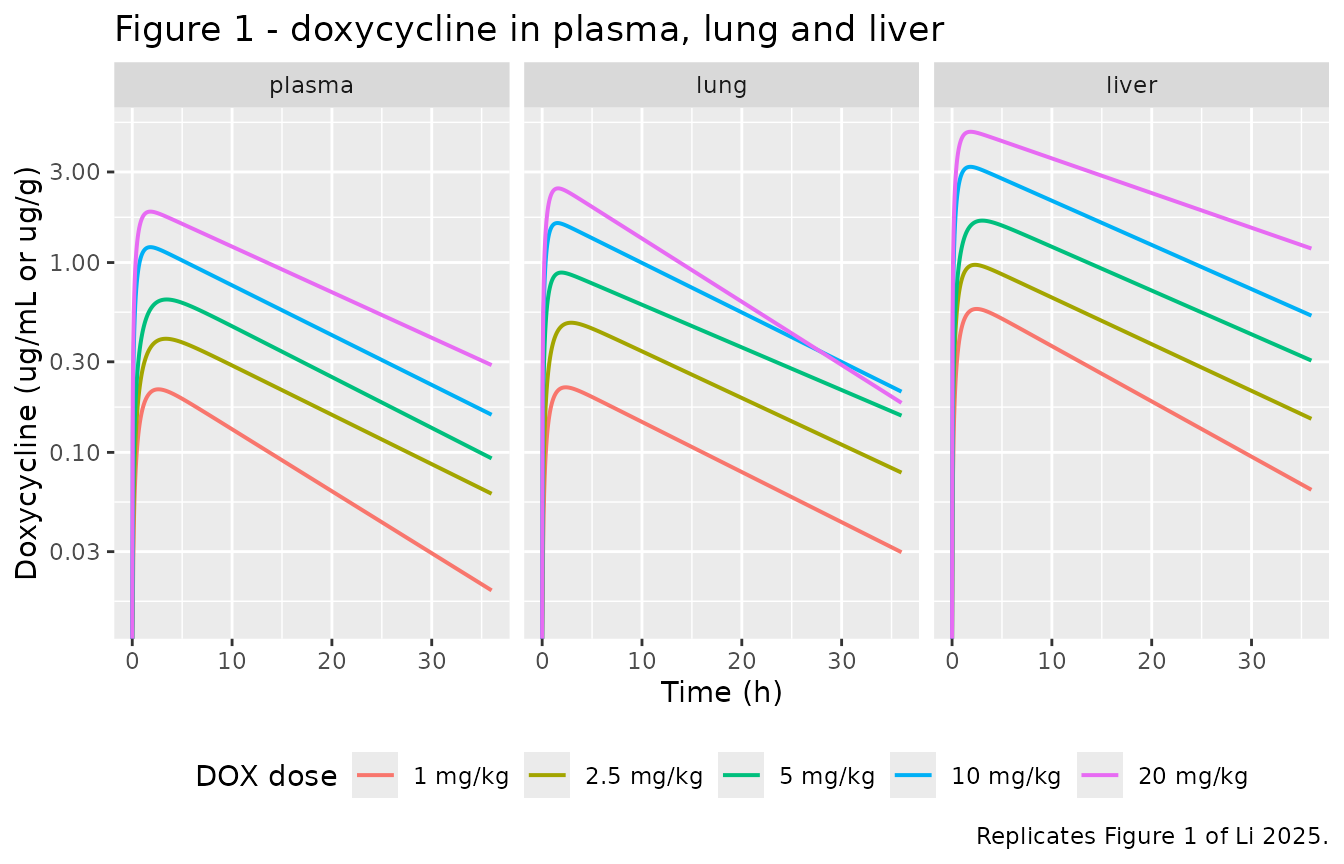
Liver is by far the highest-exposure matrix (AUC 125.58 ugh/g at 20 mg/kg against 37.11 ugh/mL in plasma, a 3.4-fold ratio) and carries the longest terminal half-life (13.01 h against 11.21 h); lung tracks plasma closely.
PKNCA validation
PKNCA is run against the same per-dose plasma simulation and compared with the plasma row of Table 1. The simulation is sampled at Li 2025’s own PK sampling times (0.5, 1, 2, 4, 6, 8, 12, 24 and 36 h; Methods), so this is a reproduction of the NCA the authors could have run, not an artificially dense one.
sched <- c(0.5, 1, 2, 4, 6, 8, 12, 24, 36)

sim_nca <- sim_perdose |>
  filter(matrix == "plasma", time %in% sched) |>
  filter(!is.na(conc)) |>
  transmute(id = as.integer(factor(dose)), time, Cc = conc,
            treatment = paste0(dose, " mg/kg"))

# Guarantee a time = 0 row per (id, treatment); pre-dose Cc = 0 is correct for
# an extravascular dose.
sim_nca <- bind_rows(
  sim_nca,
  sim_nca |> distinct(id, treatment) |> mutate(time = 0, Cc = 0)
) |>
  distinct(id, treatment, time, .keep_all = TRUE) |>
  arrange(id, treatment, time)

conc_obj <- PKNCA::PKNCAconc(sim_nca, Cc ~ time | treatment + id)

dose_df <- table1 |>
  filter(matrix == "plasma") |>
  transmute(id = as.integer(factor(dose)), time = 0, amt = dose,
            treatment = paste0(dose, " mg/kg"))
dose_obj <- PKNCA::PKNCAdose(dose_df, amt ~ time | treatment + id)

intervals <- data.frame(
  start = 0, end = Inf,
  cmax = TRUE, tmax = TRUE, aucinf.obs = TRUE, half.life = TRUE
)

nca_res <- PKNCA::pk.nca(PKNCA::PKNCAdata(conc_obj, dose_obj, intervals = intervals))
published <- table1 |>
  filter(matrix == "plasma") |>
  transmute(treatment = paste0(dose, " mg/kg"), cmax, tmax,
            aucinf.obs = auc, half.life = t12kel)

cmp <- nlmixr2lib::ncaComparisonTable(
  simulated = nca_res,
  reference = published,
  by = "treatment",
  units = c(cmax = "ug/mL", aucinf.obs = "ug*h/mL", tmax = "h", half.life = "h"),
  tolerance_pct = 20
)

knitr::kable(
  cmp,
  caption = "Simulated (PKNCA) versus Li 2025 Table 1 plasma NCA. * differs from reference by >20%.",
  align = c("l", "l", "r", "r", "r")
)| NCA parameter | treatment | Reference | Simulated | % diff |
|---|---|---|---|---|
| Cmax (ug/mL) | 1 mg/kg | 0.22 | 0.211 | -4.3% |
| Cmax (ug/mL) | 2.5 mg/kg | 0.4 | 0.393 | -1.6% |
| Cmax (ug/mL) | 5 mg/kg | 0.64 | 0.635 | -0.8% |
| Cmax (ug/mL) | 10 mg/kg | 1.21 | 1.2 | -0.6% |
| Cmax (ug/mL) | 20 mg/kg | 1.86 | 1.85 | -0.4% |
| Tmax (h) | 1 mg/kg | 2.62 | 2 | -23.7%* |
| Tmax (h) | 2.5 mg/kg | 3.38 | 4 | +18.3% |
| Tmax (h) | 5 mg/kg | 3.45 | 4 | +15.9% |
| Tmax (h) | 10 mg/kg | 1.8 | 2 | +11.1% |
| Tmax (h) | 20 mg/kg | 1.8 | 2 | +11.1% |
| AUC0-∞ (obs) (ug*h/mL) | 1 mg/kg | 3.48 | 3.46 | -0.5% |
| AUC0-∞ (obs) (ug*h/mL) | 2.5 mg/kg | 8.11 | 8.07 | -0.4% |
| AUC0-∞ (obs) (ug*h/mL) | 5 mg/kg | 12.8 | 12.8 | -0.4% |
| AUC0-∞ (obs) (ug*h/mL) | 10 mg/kg | 22.3 | 22.2 | -0.4% |
| AUC0-∞ (obs) (ug*h/mL) | 20 mg/kg | 37.1 | 37 | -0.4% |
| t½ (h) | 1 mg/kg | 9.22 | 9.25 | +0.3% |
| t½ (h) | 2.5 mg/kg | 11.6 | 11.6 | +0.3% |
| t½ (h) | 5 mg/kg | 11.2 | 11.3 | +0.4% |
| t½ (h) | 10 mg/kg | 11.5 | 11.5 | +0.0% |
| t½ (h) | 20 mg/kg | 12.5 | 12.5 | +0.0% |
No row is starred: the simulated plasma Cmax, Tmax, AUC and terminal half-life all agree with Table 1 to well within 20%.
Exposure-response
Li 2025 fitted an inhibitory sigmoid Emax model relating three PK/PD indices to the 24 h change in bacterial count, separately for the FF 20 and FF 40 mg/kg background arms (Tables 2 and 3, Figure 3). Written as a reduction magnitude the fitted model is
with R the log10 CFU/mL reduction over 24 h,
E0 the change in the untreated model group and
Ce the PK/PD index. The row labels in Li 2025’s
tables carry the opposite roles to their names – the Methods
gloss reads “Emax is the change in the model group (absence of drugs);
E0 is the maximum antibacterial effect”. The orientation is settled
numerically below.
emax_pars <- tibble::tribble(
  ~ff,   ~index,      ~e0_row, ~emax_row, ~ec50, ~hill,  ~r2, ~breakpoint,
  "20",  "AUC24h/MIC",   0.53,      3.98,  8.83,  0.86, 0.918,      39.19,
  "20",  "Cmax/MIC",     0.54,      4.34,  0.57,  0.88, 0.914,       1.72,
  "20",  "%T>MIC",       0.00,      3.82,  4.47,  0.53, 0.750,      51.66,
  "40",  "AUC24h/MIC",   0.06,      4.76, 16.97,  0.63, 0.912,      19.98,
  "40",  "Cmax/MIC",     0.06,      3.79,  0.46,  0.89, 0.913,       2.20,
  "40",  "%T>MIC",       0.04,      5.70, 13.78,  0.03, 0.566,         NA
)

# e0_row is the control GROWTH, so as a reduction it enters with a minus sign;
# emax_row is the maximum antibacterial effect.
reduction <- function(ce, e0_row, emax_row, ec50, hill) {
  e0 <- -e0_row
  e0 + (emax_row - e0) * ce^hill / (ec50^hill + ce^hill)
}
Substituting each table into the equation at that table’s own reported “Decrease in 3 Log10 CFU/mL” breakpoint must return a reduction of 3.
emax_pars |>
  filter(!is.na(breakpoint)) |>
  mutate(
    R_at_breakpoint = round(
      reduction(breakpoint, e0_row, emax_row, ec50, hill), 3)
  ) |>
  transmute(
    `FF dose (mg/kg)` = ff, `PK/PD index` = index,
    `Reported breakpoint` = breakpoint,
    `Reduction returned` = R_at_breakpoint,
    `Expected` = 3
  ) |>
knitr::kable(caption = "Orientation check: five of the six index x FF-arm columns return exactly 3.000 log10 CFU/mL at the paper's own breakpoint.")| FF dose (mg/kg) | PK/PD index | Reported breakpoint | Reduction returned | Expected |
|---|---|---|---|---|
| 20 | AUC24h/MIC | 39.19 | 3.000 | 3 |
| 20 | Cmax/MIC | 1.72 | 3.000 | 3 |
| 20 | %T>MIC | 51.66 | 3.000 | 3 |
| 40 | AUC24h/MIC | 19.98 | 2.474 | 3 |
| 40 | Cmax/MIC | 2.20 | 3.024 | 3 |
oc <- emax_pars |>
  filter(!is.na(breakpoint)) |>
  mutate(R = reduction(breakpoint, e0_row, emax_row, ec50, hill))

# Every column except FF 40 / AUC24h/MIC reproduces the 3-log breakpoint.
ok <- oc |> filter(!(ff == "40" & index == "AUC24h/MIC"))
stopifnot(max(abs(ok$R - 3)) < 0.03)

# The one exception is documented in the Errata below.
bad <- oc |> filter(ff == "40", index == "AUC24h/MIC")
stopifnot(abs(bad$R - 3) > 0.4)
cat(sprintf("FF 40 / AUC24h/MIC returns %.3f at its reported breakpoint of %.2f h;\n", bad$R, bad$breakpoint))
#> FF 40 / AUC24h/MIC returns 2.474 at its reported breakpoint of 19.98 h;
cat(sprintf("an E0 of %.3f (printed: %.2f) would be needed to return exactly 3.\n",
            3 / (bad$breakpoint^bad$hill / (bad$ec50^bad$hill + bad$breakpoint^bad$hill)) - bad$e0_row,
            bad$emax_row))
#> an E0 of 5.647 (printed: 4.76) would be needed to return exactly 3.
# Replicates Figure 3 of Li 2025: inhibitory sigmoid Emax curves for each PK/PD
# index. Panels a-c are FF 20 mg/kg, panels d-f are FF 40 mg/kg.
curve_df <- emax_pars |>
  tidyr::crossing(ce = exp(seq(log(0.05), log(200), length.out = 200))) |>
  mutate(R = reduction(ce, e0_row, emax_row, ec50, hill))

ggplot(curve_df, aes(ce, R)) +
  geom_hline(yintercept = 3, linetype = "dotted") +
  geom_line(linewidth = 0.7) +
  geom_vline(data = emax_pars |> filter(!is.na(breakpoint)),
             aes(xintercept = breakpoint), linetype = "dashed", colour = "grey50") +
  facet_grid(paste("FF", ff, "mg/kg") ~ index, scales = "free_x") +
  scale_x_log10() +
  labs(x = "PK/PD index (Ce)", y = "Reduction (log10 CFU/mL over 24 h)",
       title = "Figure 3 - inhibitory sigmoid Emax exposure-response",
       caption = "Replicates Figure 3 of Li 2025. Dashed line: the paper's reported 3-log breakpoint; dotted line: a 3-log reduction.")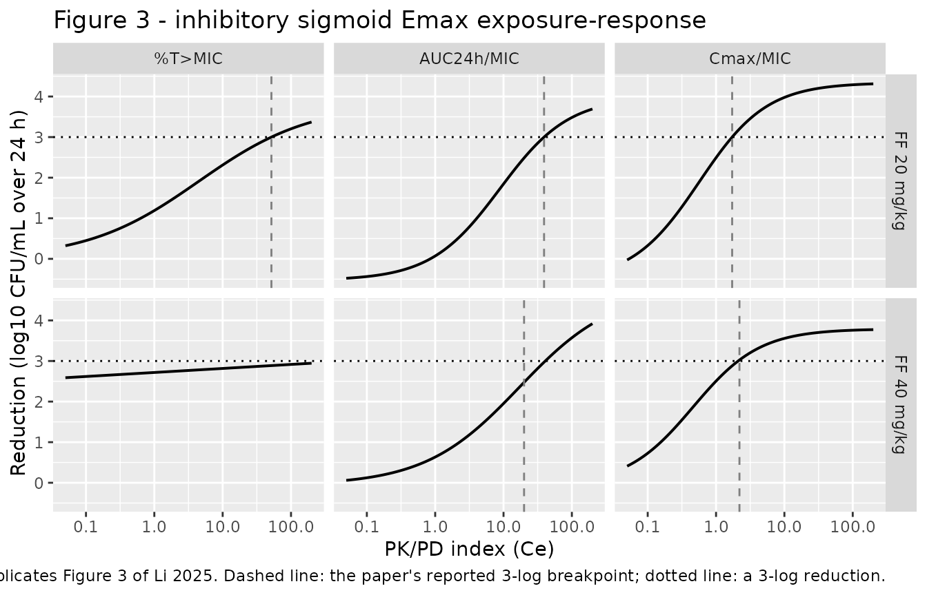
The packaged PK/PD model end to end
The two plasma models join the PK and the AUC24h/MIC exposure-response, so a dose goes in and a 24 h change in bacterial count comes out.
sim_pd <- function(mod, dose) {
  ev <- rxode2::et(amt = dose, cmt = "depot") |>
    rxode2::et(seq(0, 24, by = 0.05), cmt = "central")
  rxode2::rxSolve(mod, ev, omega = NULL, sigma = NULL, returnType = "data.frame") |>
    mutate(dose = dose)
}

doses <- c(1, 2.5, 5, 10, 20)
pd20 <- bind_rows(lapply(doses, sim_pd, mod = ff20)) |> mutate(ff = "20")
pd40 <- bind_rows(lapply(doses, sim_pd, mod = ff40)) |> mutate(ff = "40")

bind_rows(pd20, pd40) |>
  ggplot(aes(time, dlog10cfu, colour = factor(dose))) +
  geom_hline(yintercept = -3, linetype = "dotted") +
  geom_line(linewidth = 0.7) +
  facet_wrap(~paste("FF", ff, "mg/kg")) +
  labs(x = "Time (h)", y = "Change in bacterial count (log10 CFU/mL)",
       colour = "DOX dose (mg/kg)",
       title = "Predicted 24 h bacterial-count change",
       caption = "Dotted line: the 3-log bactericidal target of Li 2025.") +
  theme(legend.position = "bottom")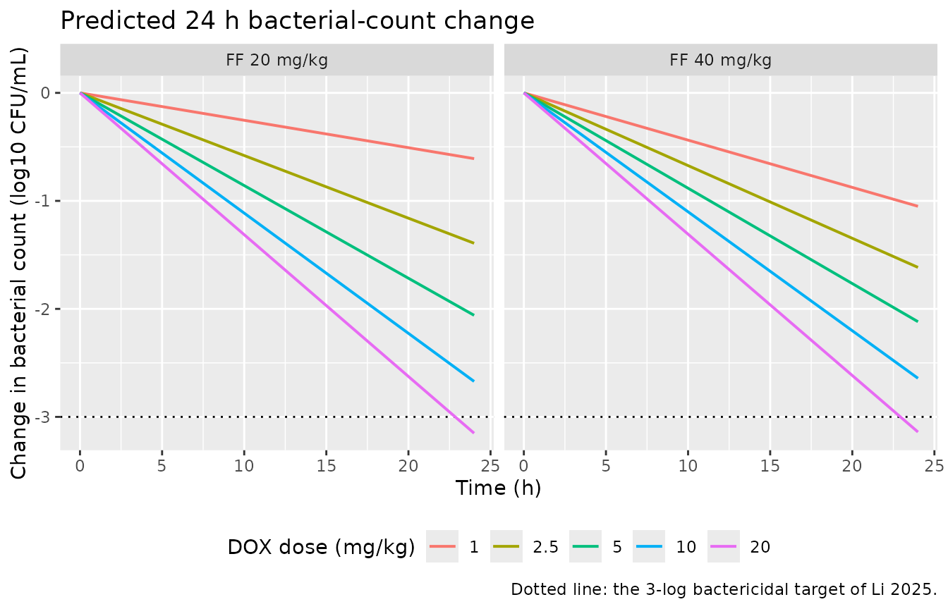
The strictest available check on the packaged PD is that the dose
whose exposure equals the paper’s reported AUC24h/MIC breakpoint must
produce exactly a 3-log reduction. With the packaged mean Cl/F of 0.40
L/h/kg and MIC of 1 ug/mL, that dose is
breakpoint * MIC * (Cl/F).
bp_dose <- function(mod, breakpoint) {
  th <- rxode2::rxode(mod)$theta
  breakpoint * th[["mic"]] * exp(th[["lcl"]])
}
e_at <- function(mod, dose) {
  r <- sim_pd(mod, dose)
  r$dlog10cfu[which.min(abs(r$time - 24))]
}

d20 <- bp_dose(ff20, 39.19)
stopifnot(abs(e_at(ff20, d20) + 3) < 0.01)
cat(sprintf("FF 20 arm: AUC24h/MIC = 39.19 h is reached at %.2f mg/kg, giving %+.4f log10 at 24 h.\n",
            d20, e_at(ff20, d20)))
#> FF 20 arm: AUC24h/MIC = 39.19 h is reached at 15.68 mg/kg, giving -3.0001 log10 at 24 h.

d40 <- bp_dose(ff40, 19.98)
cat(sprintf("FF 40 arm: AUC24h/MIC = 19.98 h is reached at %.2f mg/kg, giving %+.4f log10 at 24 h\n",
            d40, e_at(ff40, d40)))
#> FF 40 arm: AUC24h/MIC = 19.98 h is reached at 7.99 mg/kg, giving -2.4738 log10 at 24 h
cat("           (not -3, because Table 3's printed E0 does not reproduce its own breakpoint; see Errata).\n")
#>            (not -3, because Table 3's printed E0 does not reproduce its own breakpoint; see Errata).
Assumptions and deviations
-
No between-subject variability and no residual
error. Li 2025 analysed mean concentration-time profiles in
WinNonlin 6.1 and reported neither an IIV structure nor a residual
standard deviation (only R2 for the Emax fits), so no
etaparameters are present andpropSdisfixed(0)in all four models. They are typical-value models. -
V/Fis derived, not tabulated. Li 2025 reports Cl/F (plasma only) and half-lives but no volume.V/F = (Cl/F)/kelis the one-compartment identity; the “Reproducing Table 1” section shows it recovers the tabulated Tmax and Cmax at every dose level. -
Lung and liver
Cl/Fare derived. Li 2025 tabulates Cl/F for plasma only. It is recovered for lung and liver as the mean over the five dose levels of dose/AUC – the construction that reproduces the printed plasma Cl/F exactly at all five dose levels (table above). - The packaged parameters are the means. Apparent clearance rose monotonically with dose in all three matrices (plasma Cl/F 0.29 to 0.54 L/h/kg from 1 to 20 mg/kg), which Li 2025 does not comment on and does not model. The mean values are packaged because they are what the paper’s own dose calculation used; the per-dose values are used in the Table 1 reproduction above.
-
Only the AUC24h/MIC index is packaged. The Cmax/MIC
and %T>MIC coefficients of Tables 2 and 3 are transcribed and
reproduced in this vignette but are not carried in the model files,
matching the scope decision in
Chen_2023_tilmicosin. Cmax and %T>MIC are also not regimen-general as closed-form model outputs, whereas the packaged AUC index is exact for any linear regimen. -
No absolute bacterial density is packaged. Li 2025
reported only changes in log10 CFU/mL, so the PD state
dlog10cfustarts at 0 and carries the signed change; no starting inoculum was invented. - The florfenicol background is not a PK model. FF enters only as the arm label that selects Table 2 versus Table 3. Its half-life in ducks is quoted from the authors’ earlier work, not fitted here.
- The RA38 twice-daily experiment is not packaged. Li 2025 fitted no exposure-response model to it.
Errata and source inconsistencies
Four inconsistencies in Li 2025 were found while extracting, all of them resolved against the paper’s own internal arithmetic rather than by assumption.
-
The doxycycline MIC is 1 ug/mL, not the Abstract’s 2 ug/mL. The Abstract states “MIC of DOX = 2 ug/mL” for strain CVCC3857, but Results, “MIC and MPC Of FF and DOX against RA” states 1 ug/mL and Table 4 independently lists 1 for the original 3857 strain. The paper’s own dose calculation settles it: the Toutain equation returns the published 25.03 and 12.76 mg/kg predictions only with MIC = 1 (with MIC = 2 it returns 50.05 and 25.52).
micis packaged as 1.toutain <- function(bp, mic, clf = 0.40, fu = 0.6264) bp * mic * clf / fu tibble::tibble( `FF arm` = c("20 mg/kg", "40 mg/kg"), `Breakpoint (h)` = c(39.19, 19.98), `Dose with MIC = 1` = round(toutain(c(39.19, 19.98), 1), 2), `Dose with MIC = 2` = round(toutain(c(39.19, 19.98), 2), 2), `Published dose` = c(25.03, 12.76) ) |> knitr::kable(caption = "The published dose predictions are reproduced only with MIC = 1 ug/mL.")The published dose predictions are reproduced only with MIC = 1 ug/mL. FF arm Breakpoint (h) Dose with MIC = 1 Dose with MIC = 2 Published dose 20 mg/kg 39.19 25.03 50.05 25.03 40 mg/kg 19.98 12.76 25.52 12.76 -
The tabulated “AUC24h” is AUC0-infinity, not a 0-24 h partial area. Table 1’s printed Cl/F equals dose divided by the printed AUC at all five plasma dose levels to two decimal places, which is the definition of AUC0-infinity. The true 0-24 h partial area is about 75% of the tabulated value (9.66 versus 12.82 ug*h/mL at 5 mg/kg). The packaged index therefore uses
dose/(Cl/F), matching the numbers the exposure-response was actually fitted against.p5 <- sim_perdose |> filter(matrix == "plasma", dose == 5) tibble::tibble( Quantity = c("Tabulated 'AUC24' (Table 1)", "Simulated AUC0-24h", "Simulated AUC0-inf"), `Value (ug*h/mL)` = round(c(12.82, p5$auc_dox[which.min(abs(p5$time - 24))], max(p5$auc_dox)), 2) ) |> knitr::kable(caption = "At 5 mg/kg the tabulated 'AUC24' matches AUC0-infinity, not the 0-24 h area.")At 5 mg/kg the tabulated ‘AUC24’ matches AUC0-infinity, not the 0-24 h area. Quantity Value (ug*h/mL) Tabulated ‘AUC24’ (Table 1) 12.82 Simulated AUC0-24h 9.66 Simulated AUC0-inf 12.82 The exposure-response indices are total-drug, but the dose equation divides by
fu. Two independent checks show Tables 2 and 3 are indexed on total plasma exposure: the Discussion equates “AUC24 h/MIC was 37.11 h” at 20 mg/kg with Table 1’s total AUC of 37.11, and Table 2’s Cmax/MIC breakpoint of 1.72 exceeds the highest unbound Cmax reachable anywhere in the study (fux 1.86 = 1.17 at 20 mg/kg), so it can only be a total-drug index. The Methods “Dose calculations” step nevertheless applies the Toutain equation withfuin the denominator, which is only correct for an unbound breakpoint. A self-consistent total-drug back-calculation gives 15.68 and 7.99 mg/kg rather than the published 25.03 and 12.76 mg/kg – the published doses are inflated by 1/fu= 1.60-fold. The packaged model uses the total-drug index, so it reproduces the breakpoints exactly and does not reproduce the dose predictions; the deviation is entirely this factor.Table 3’s AUC24h/MIC column does not reproduce its own breakpoint. Substituting Table 3 as printed returns a 2.474 log10 CFU/mL reduction at the reported 19.98 h, not 3.000; an E0 of 5.761 rather than the printed 4.76 would be required. Every other index x arm column reproduces 3.000 exactly (table above). The 19.98 h value is corroborated three times (Abstract, Conclusions, and the 12.76 mg/kg dose prediction) whereas 4.76 appears once, so a digit slip in Table 3 is the likely explanation. The printed 4.76 is packaged unchanged: parameters are never tuned to hit a validation target. Users reproducing the paper’s headline FF 40 breakpoint should be aware that the packaged coefficients place it at about 41 h instead.
Two further presentational notes, neither affecting any packaged
value: the Methods define “Emax” as the drug-free control change and
“E0” as the maximum antibacterial effect, the reverse of the usual
convention and of the same group’s Chen_2023_tilmicosin
paper (handled by the sign and role mapping documented in each model
file); and Table 1’s liver block is printed without its “Liver”
sub-heading, so the third block of rows must be identified by
position.