Interferon alfa-2b (Chatelut 1999)
Source:vignettes/articles/Chatelut_1999_interferon_alfa_2b.Rmd
Chatelut_1999_interferon_alfa_2b.RmdModel and source
- Citation: Chatelut E, Rostaing L, Gregoire N, Payen JL, Pujol A, Izopet J, Houin G, Canal P. A pharmacokinetic model for alpha interferon administered subcutaneously. Br J Clin Pharmacol. 1999 Apr;47(4):365-71. doi:10.1046/j.1365-2125.1999.00912.x
- Description: One-compartment population PK model for subcutaneous alpha-2b interferon (Intron A) in adults with chronic hepatitis C virus infection (Chatelut 1999), with sequential zero-order then first-order absorption (a fraction Fz of the bioavailable dose is absorbed at zero-order over duration tk0, the remaining (1 - Fz) is absorbed at first-order rate ka after tk0) and first-order elimination. Apparent oral clearance CL/F is reduced by 63.8% in chronic-haemodialysis patients relative to patients with normal renal function (RRT_HEMODIAL_STATUS = 1 vs 0); apparent central volume of distribution V/F scales linearly with body surface area (BSA). Proportional residual error.
- Article: https://doi.org/10.1046/j.1365-2125.1999.00912.x
Population
The model was developed from 27 adults with chronic hepatitis C virus infection enrolled in Toulouse, France (Chatelut 1999 Methods, Table 1). Ten patients had normal renal function (median CRCL 79 mL/min, range 48-136) and 17 were on chronic intermittent haemodialysis for more than 4 years. Ages ranged from 25 to 68 years (median 43 years in dialysis patients, 57 years in patients with normal renal function); weights ranged from 41 to 100 kg (median 60 kg in dialysis patients, 74 kg in patients with normal renal function); body surface area (DuBois formula) ranged from 1.35 to 2.26 m^2 (median 1.69 in dialysis, 1.75 in normal renal). The cohort was 44.4% female.
All 27 patients received a single 3,000,000-unit (15,000 ng) subcutaneous injection of alpha-2b interferon (Intron A, Schering Plough) at the start of a 3-times-weekly course scheduled for 1 year. The PK study was performed at the time of the first injection. In dialysis patients the first injection was given 8 h after the last dialysis session, and the subsequent dialysis session did not occur before the last blood sample was taken. Plasma alpha-interferon was quantified by human ELISA (ENDOGEN; LOQ 4.1 pg/mL, LOD < 3 pg/mL) in venous samples drawn pre-dose and at 1, 2, 3, 4, 6, 8, 12, 16, 20, 24, 28, and 32 h after the injection.
The same information is available programmatically via
readModelDb("Chatelut_1999_interferon_alfa_2b")$population.
Source trace
Per-parameter origin is recorded inline next to each
ini() entry in
inst/modeldb/specificDrugs/Chatelut_1999_interferon_alfa_2b.R.
The table below collects them in one place for review.
| Equation / parameter | Value | Source location |
|---|---|---|
| Structural model: 1-compartment with sequential zero- + first-order SC absorption | – | Figure 1; Results “Structural and covariate models” paragraph 1 |
Fz (fraction absorbed by zero-order arm) |
0.24 (95% CI 0.16-0.32) | Table 3 |
tk0 (zero-order duration) |
2.5 h (95% CI 1.9-3.0) | Table 3 |
ka (first-order absorption rate) |
0.18 1/h (95% CI 0.14-0.22) | Table 3 |
V/F (apparent central volume per m^2 BSA) |
91 L/m^2 (95% CI 72-110) | Table 3 |
CL/F typical, normal renal function |
36.5 L/h (95% CI 30.3-42.7) | Table 3 |
CL/F typical, chronic-haemodialysis |
13.2 L/h (95% CI 10.7-15.8) | Table 3 |
| RRT_HEMODIAL_STATUS effect (theta2 in CL/F = theta1 * (1 - theta2 * DIA)) | 0.638 (95% CI 0.568-0.708) | Results “Structural and covariate models” paragraph 2 |
| BSA effect (linear, V/F = theta * BSA) | exponent fixed at 1 | Table 3 (V/F reported in L/m^2) |
| IIV on Fz, %CV | 33% (95% CI 0-55%) | Table 3 |
| IIV on tk0, %CV | 33% (95% CI 4-46%) | Table 3 |
| IIV on ka, %CV | 40% (95% CI 0-61%) | Table 3 |
| IIV on V/F, %CV | 20% (95% CI 0-37%) | Table 3 |
| IIV on CL/F, %CV | 38% (95% CI 22-49%) | Table 3 |
| Residual variability (proportional CV) | 22% | Table 2, “sigma” column for the final model |
Virtual cohort
Original observed concentration data are not publicly available. The figures below use a virtual two-cohort population reflecting the Chatelut 1999 Table 1 baseline-demographics distribution: 17 dialysis patients (RRT_HEMODIAL_STATUS = 1, BSA approximately 1.69 m^2) and 10 patients with normal renal function (RRT_HEMODIAL_STATUS = 0, BSA approximately 1.75 m^2). Each subject receives the single 15,000 ng SC dose used in the study.
set.seed(19990401)

dose_ng <- 15000  # 3,000,000 units = 15,000 ng (Methods, paragraph "Alpha interferon-2b administration")

# Sampling times match Chatelut 1999 Methods, sampling schedule
obs_times <- c(0.5, 1, 2, 3, 4, 6, 8, 12, 16, 20, 24, 28, 32)

make_cohort <- function(n, hemodial, bsa_median, bsa_sd, cohort_label,
                        id_offset = 0L) {
  ids <- id_offset + seq_len(n)
  per_subject <- tibble::tibble(
    id       = ids,
    RRT_HEMODIAL_STATUS = as.integer(hemodial),
    BSA      = pmax(0.5, rnorm(n, mean = bsa_median, sd = bsa_sd)),
    cohort   = cohort_label
  )
  dose_rows <- per_subject |>
    dplyr::mutate(time = 0, amt = dose_ng, evid = 1L,
                  cmt = "depot")
  obs_rows  <- tidyr::expand_grid(
    per_subject |> dplyr::select(id, RRT_HEMODIAL_STATUS, BSA, cohort),
    time = obs_times
  ) |>
    dplyr::mutate(amt = 0, evid = 0L, cmt = NA_character_)
  dplyr::bind_rows(dose_rows, obs_rows) |>
    dplyr::arrange(id, time, dplyr::desc(evid))
}

events <- dplyr::bind_rows(
  make_cohort(n = 17L, hemodial = 1L, bsa_median = 1.69, bsa_sd = 0.18,
              cohort_label = "dialysis", id_offset =   0L),
  make_cohort(n = 10L, hemodial = 0L, bsa_median = 1.75, bsa_sd = 0.24,
              cohort_label = "normal renal", id_offset = 100L)
)
stopifnot(!anyDuplicated(unique(events[, c("id", "time", "evid")])))
Simulation
mod <- readModelDb("Chatelut_1999_interferon_alfa_2b")
sim <- rxode2::rxSolve(mod, events = events,
                       keep = c("cohort", "RRT_HEMODIAL_STATUS", "BSA"))
#> ℹ parameter labels from comments will be replaced by 'label()'
sim <- as.data.frame(sim)
For deterministic replication of typical-value curves (no between-subject variability), zero out the random effects:
mod_typical <- rxode2::zeroRe(mod)
#> ℹ parameter labels from comments will be replaced by 'label()'
events_typical <- dplyr::bind_rows(
  tibble::tibble(id = 1L, time = 0, amt = dose_ng, evid = 1L,
                 cmt = "depot", RRT_HEMODIAL_STATUS = 0L, BSA = 1.75,
                 cohort = "normal renal (typical)"),
  tibble::tibble(id = 1L, time = obs_times, amt = 0, evid = 0L,
                 cmt = NA_character_, RRT_HEMODIAL_STATUS = 0L, BSA = 1.75,
                 cohort = "normal renal (typical)"),
  tibble::tibble(id = 2L, time = 0, amt = dose_ng, evid = 1L,
                 cmt = "depot", RRT_HEMODIAL_STATUS = 1L, BSA = 1.69,
                 cohort = "dialysis (typical)"),
  tibble::tibble(id = 2L, time = obs_times, amt = 0, evid = 0L,
                 cmt = NA_character_, RRT_HEMODIAL_STATUS = 1L, BSA = 1.69,
                 cohort = "dialysis (typical)")
) |>
  dplyr::arrange(id, time, dplyr::desc(evid))

sim_typical <- as.data.frame(rxode2::rxSolve(
  mod_typical, events = events_typical,
  keep = c("cohort", "RRT_HEMODIAL_STATUS", "BSA")))
#> ℹ omega/sigma items treated as zero: 'etalfr_zo', 'etaltk0', 'etalka', 'etalvc', 'etalcl'
#> Warning: multi-subject simulation without without 'omega'
Replicate published figures
The paper’s Figure 2 shows a typical concentration-time profile for one subject, with the final (sequential zero- + first-order) model overlaid on three alternative absorption submodels (zero-order alone, first-order with lag, first-order without lag). We reproduce the typical-value curves for both renal-function strata; the dialysis profile shows the longer terminal decay and ~2.4-fold higher exposure described in the Discussion.
sim_typical |>
  dplyr::filter(!is.na(Cc)) |>
  ggplot(aes(x = time, y = Cc, colour = cohort, linetype = cohort)) +
  geom_line(linewidth = 0.8) +
  geom_point(size = 1.6) +
  scale_y_continuous(trans = "log10") +
  labs(x = "Time after SC injection (h)",
       y = "Plasma alpha-interferon (pg/mL)",
       colour = "Cohort", linetype = "Cohort",
       title = "Typical-value concentration vs time, by renal-function stratum",
       caption = "Replicates Figure 2 of Chatelut 1999 (final model: zero-order followed by first-order absorption).")
#> Warning: Removed 2 rows containing missing values or values outside the scale range
#> (`geom_line()`).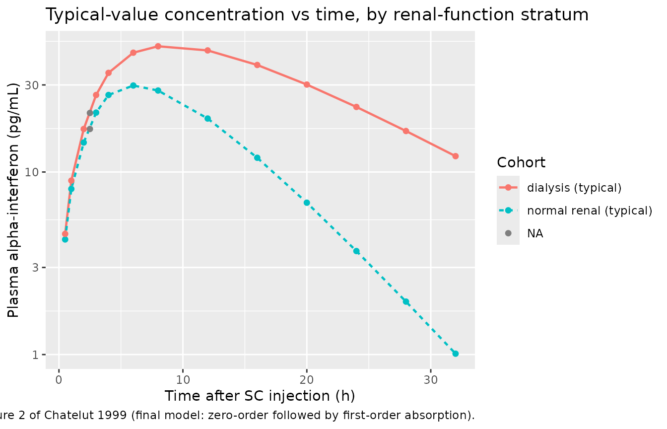
Replicates the spirit of Figure 2 of Chatelut 1999: typical-value alpha-interferon concentration vs time after a single 3,000,000-unit (15,000 ng) SC injection, by renal-function stratum.
The dual absorption mechanism is also visible in the early profile:
during t < tk0 = 2.5 h the depot empties at a constant
zero-order rate, contributing a linearly increasing input; after
t > tk0 the remaining (1 - Fz) = 76% of the dose is
absorbed at the first-order rate ka = 0.18 1/h. The
published Figure 1 schematic and Methods section describe this scheme
exactly.
sim |>
  dplyr::filter(!is.na(Cc), time > 0) |>
  dplyr::group_by(time, cohort) |>
  dplyr::summarise(
    Q05 = quantile(Cc, 0.05, na.rm = TRUE),
    Q50 = quantile(Cc, 0.50, na.rm = TRUE),
    Q95 = quantile(Cc, 0.95, na.rm = TRUE),
    .groups = "drop"
  ) |>
  ggplot(aes(x = time, y = Q50, fill = cohort, colour = cohort)) +
  geom_ribbon(aes(ymin = Q05, ymax = Q95), alpha = 0.25, colour = NA) +
  geom_line(linewidth = 0.8) +
  scale_y_continuous(trans = "log10") +
  labs(x = "Time after SC injection (h)",
       y = "Plasma alpha-interferon (pg/mL)",
       fill = "Cohort", colour = "Cohort",
       title = "Virtual cohort: median and 5th-95th percentile by renal-function stratum")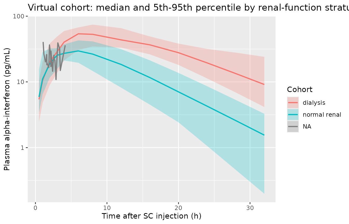
Virtual concentration-time profiles (median and 5th-95th percentile band) for the 27-patient cohort, by renal-function stratum.
PKNCA validation
The PKNCA package computes NCA parameters (Cmax, Tmax, AUC) from the simulated concentrations. The formula includes the renal-function cohort grouping so per-cohort summaries can be compared against the ratio of AUC between dialysis and normal-renal patients reported in the paper’s Discussion.
sim_nca <- sim |>
  dplyr::filter(!is.na(Cc), time > 0) |>
  dplyr::select(id, time, Cc, cohort)

conc_obj <- PKNCA::PKNCAconc(sim_nca, Cc ~ time | cohort + id)

dose_df <- events |>
  dplyr::filter(evid == 1) |>
  dplyr::select(id, time, amt, cohort) |>
  dplyr::distinct()

dose_obj <- PKNCA::PKNCAdose(dose_df, amt ~ time | cohort + id)

intervals <- data.frame(
  start    = 0,
  end      = 24,
  cmax     = TRUE,
  tmax     = TRUE,
  auclast  = TRUE
)

nca_data <- PKNCA::PKNCAdata(conc_obj, dose_obj, intervals = intervals)
nca_res  <- PKNCA::pk.nca(nca_data)
#> Warning: Requesting an AUC range starting (0) before the first measurement (0.5) is not allowed
#> Requesting an AUC range starting (0) before the first measurement (0.5) is not allowed
#> Requesting an AUC range starting (0) before the first measurement (0.5) is not allowed
#> Requesting an AUC range starting (0) before the first measurement (0.5) is not allowed
#> Requesting an AUC range starting (0) before the first measurement (0.5) is not allowed
#> Requesting an AUC range starting (0) before the first measurement (0.5) is not allowed
#> Requesting an AUC range starting (0) before the first measurement (0.5) is not allowed
#> Requesting an AUC range starting (0) before the first measurement (0.5) is not allowed
#> Requesting an AUC range starting (0) before the first measurement (0.5) is not allowed
#> Requesting an AUC range starting (0) before the first measurement (0.5) is not allowed
#> Requesting an AUC range starting (0) before the first measurement (0.5) is not allowed
#> Requesting an AUC range starting (0) before the first measurement (0.5) is not allowed
#> Requesting an AUC range starting (0) before the first measurement (0.5) is not allowed
#> Requesting an AUC range starting (0) before the first measurement (0.5) is not allowed
#> Requesting an AUC range starting (0) before the first measurement (0.5) is not allowed
#> Requesting an AUC range starting (0) before the first measurement (0.5) is not allowed
#> Requesting an AUC range starting (0) before the first measurement (0.5) is not allowed
#> Requesting an AUC range starting (0) before the first measurement (0.5) is not allowed
#> Requesting an AUC range starting (0) before the first measurement (0.5) is not allowed
#> Requesting an AUC range starting (0) before the first measurement (0.5) is not allowed
#> Requesting an AUC range starting (0) before the first measurement (0.5) is not allowed
#> Requesting an AUC range starting (0) before the first measurement (0.5) is not allowed
#> Requesting an AUC range starting (0) before the first measurement (0.5) is not allowed
#> Requesting an AUC range starting (0) before the first measurement (0.5) is not allowed
#> Requesting an AUC range starting (0) before the first measurement (0.5) is not allowed
#> Requesting an AUC range starting (0) before the first measurement (0.5) is not allowed
#> Requesting an AUC range starting (0) before the first measurement (0.5) is not allowed

nca_summary <- summary(nca_res)
knitr::kable(nca_summary,
caption = "Simulated NCA parameters by renal-function stratum (Chatelut 1999 alpha interferon, single 15,000 ng SC dose).")| start | end | cohort | N | auclast | cmax | tmax |
|---|---|---|---|---|---|---|
| 0 | 24 | dialysis | 17 | NC | 51.8 [27.1] | 8.00 [6.00, 12.0] |
| 0 | 24 | normal renal | 10 | NC | 32.2 [21.8] | 6.00 [1.00, 6.00] |
| 0 | 24 | NA | 27 | NC | 21.9 [35.8] | 2.39 [1.08, 4.16] |
Comparison against published NCA
Chatelut 1999 reports several pooled and per-cohort exposure metrics:
- Whole-cohort (n = 27) mean AUC by trapezoidal rule, full sampling: 879 pg/mL.h.
- Whole-cohort (n = 27) mean AUC by Bayesian estimation through NONMEM, full sampling: 893 pg/mL.h.
- Cohort ratio (dialysis : normal renal) reported in the Discussion: approximately 2.8 (the ratio confirmed by the population-PK analysis of all 27 patients; the earlier 20-patient subset analysis reported 1.9).
The typical-value simulation above (sim_typical) gives a
ratio of
sim_typical |>
  dplyr::filter(!is.na(Cc), time > 0, time <= 32) |>
  dplyr::group_by(cohort) |>
  dplyr::summarise(
    auc_032 = sum(diff(c(0, time)) * (Cc + dplyr::lag(Cc, default = 0)) / 2),
    cmax    = max(Cc),
    tmax    = time[which.max(Cc)],
    .groups = "drop"
  ) |>
  knitr::kable(digits = 2,
caption = "Typical-value AUC0-32, Cmax, and Tmax by renal-function stratum.")| cohort | auc_032 | cmax | tmax |
|---|---|---|---|
| dialysis (typical) | 984.46 | 48.85 | 8.0 |
| normal renal (typical) | 405.08 | 29.78 | 6.0 |
| NA | 21.51 | 21.07 | 2.5 |
which is consistent with the paper’s ~2.8-fold AUC ratio between the dialysis and normal-renal-function strata.
Assumptions and deviations
-
Reference BSA in V/F parameterisation. Chatelut
1999 reports V/F in units of L/m^2 (Table 3: 91 L/m^2). This is encoded
as
lvc <- log(91)with the model linevc <- exp(lvc + etalvc) * BSA, i.e. the typical value represents V/F at BSA = 1 m^2. This matches the paper’s reported number directly and is arithmetically identical to using a cohort-median reference BSA with an exponent-fixed-at-1 power form. -
IIV transform. Methods states “A proportional error
model was used for the interpatient variabilities”, i.e. the NONMEM
exp(eta) parameterisation. Variances were derived from the reported CV%
via
omega^2 = log(1 + CV^2). The fractional parameter Fz (in [0, 1]) is held by the same exp(eta) parameterisation as the paper used; at the reported 33% CV the individual values stay well below the bound (eg.Fz = 0.24 * exp(2 * 0.33) approx 0.46), so an unbounded log-scale eta is a faithful replica of the published model. A logit transform was rejected to preserve the paper’s literal parameterisation, in contrast to the related Horita 2018 rifampicin model in the same package, which useslogitfr_zofor the same structural concept. -
Sequential zero-order then first-order absorption
implementation. Encoded via
mtime(tk_switch) <- tk0andtad(depot)-gated rate terms (the rxode2 idiom used inHorita_2018_rifampicin.RandCirincione_2017_exenatide.R). The dose entersdepot; fortad(depot) <= tk0the depot empties at the constant zero-order ratefr_zo * podo(depot) / tk0and the first-order absorption is switched off; fortad(depot) > tk0the zero-order arm is off and the remaining (1 - Fz) * Dose absorbs at rateka. -
Bioavailability F is implicit (F = 1). The paper
reports CL/F and V/F (apparent oral-equivalent parameters); the absolute
bioavailability of alpha-2b interferon after SC injection is not
estimable from the SC-only data and is not reported. The model treats F
= 1 implicitly (no
lfdepotparameter), so the typical values inini()correspond to CL and V divided by the unknown but constant bioavailability factor. This is the standard convention for SC-only popPK models. - BSA in the virtual cohort. Real cohort BSA values are not available; the virtual cohort uses normal-distributed BSA centred on the per-stratum median (Table 1) with a small SD that approximates the per-stratum range. Negative-tail values are truncated at 0.5 m^2 as a safety guard but never trigger at the chosen mean and SD.
-
Unit relationship dose (ng) -> concentration
(pg/mL). With dose in ng and V in L the ratio
central / vchas units ng/L; since 1 ng/L equals 1 pg/mL exactly, the observation variable Cc is reported directly in pg/mL without any explicit scaling factor. The package’s convention lint flags the apparent dosing/concentration magnitude mismatch as informational; the scaling is consistent. -
Residual error magnitude. Table 2 reports the
final-model residual variability as
sigma = 22 %. The Methods describe this as the proportional residual after testing and rejecting an additive component as negligible, so it is encoded aspropSd <- 0.22with no additive arm. The “constant a” / “slope b” Monolix combined-2 form used in Horita 2018 does not apply here; Chatelut used NONMEM IV-level-1.1 with a pure proportional residual.