Tepotinib and MSC2571109A (Xiong 2022)
Source:vignettes/articles/Xiong_2022_tepotinib.Rmd
Xiong_2022_tepotinib.RmdModel and source
- Citation: Xiong W, Papasouliotis O, Jonsson EN, Strotmann R, Girard P. Population pharmacokinetic analysis of tepotinib, an oral MET kinase inhibitor, including data from the VISION study. Cancer Chemother Pharmacol. 2022;89(5):655-669. doi:10.1007/s00280-022-04423-5. PMCID PMC9054876. Parameter values from Table 3; covariate-model functional forms from Electronic Supplementary Material ESM 13.
- Description: Two-compartment population PK model for oral tepotinib with sequential zero- then first-order absorption and first-order elimination, linked to a two-compartment model for its major circulating metabolite MSC2571109A (formed from parent clearance, fraction metabolised fixed to 1), in patients with cancer (including MET exon 14 skipping NSCLC from VISION) and healthy participants pooled from 12 studies. Dose-dependent relative bioavailability; food, formulation, hepatic dysfunction, eGFR, tumour type, opioid co-medication, INR and serum albumin covariates.
- Article: https://doi.org/10.1007/s00280-022-04423-5 (open access, CC BY 4.0)
- Supplement: Electronic Supplementary Material ESM 1-13 at the article landing page.
Tepotinib is a once-daily oral MET kinase inhibitor approved for non-small cell lung cancer (NSCLC) with MET exon 14 skipping. Xiong et al. pooled 12 studies and fitted the parent drug first, then fitted its major circulating metabolite MSC2571109A with the individual tepotinib parameters held fixed (sequential approach). Both analytes live in one model file here because the metabolite is formed from the parent’s clearance and cannot be simulated without it.
Population
The tepotinib analysis set (Table 2) had 613 participants and 10,788 concentrations: 438 patients with cancer (NSCLC, including MET exon 14 skipping NSCLC from the pivotal VISION study, hepatocellular carcinoma, colorectal, renal cell, gastroesophageal and other solid tumours) and 175 healthy participants, some with mild or moderate hepatic impairment. Median age was 58 years (range 18-89), median weight 72.0 kg (35.5-136), 174 (28%) were female, and race was 59% Caucasian, 5% Japanese, 24% other East Asian, 3% African origin, 4% Hispanic and 6% other or missing. Doses ranged from 30 to 1400 mg/day as capsules (CF1 non-micronised, CF2 micronised) or tablets (TF1, TF1* finely micronised, TF2, TF3), given once daily, three times weekly or as a single dose, fasted or fed. The MSC2571109A set had 464 participants and 7197 concentrations.
The same information is available programmatically via
readModelDb("Xiong_2022_tepotinib")()$population.
Source trace
Values come from Table 3 of the article; the functional form of every
covariate relationship comes from ESM 13, which writes the final
tepotinib covariate model out in full. The metabolite covariate forms
follow the Methods’ Formula 1 (power model on continuous covariates,
normalised to the reference value) and Formula 2 (fractional difference,
1 + theta, for a categorical covariate), the same forms ESM
13 uses for the parent.
| Equation / parameter | Value | Source location |
|---|---|---|
Structure: 2-cmt parent, zero-order input of duration D1 into the
depot then first-order ka; 2-cmt metabolite formed from
fm * CL/Vc * central
|
n/a | Results; Figure 1 |
lcl (CL/F) |
20.4 L/h | Table 3; ESM 13 |
lvc (Vc/F) |
1020 L | Table 3 (ESM 13 prints 1030; see Assumptions) |
lka (ka) |
0.278 1/h | Table 3 (ESM 13 prints 1.47; see the ka check below) |
lq (Q/F) |
1.32 L/h | Table 3; ESM 13 |
lvp (Vp/F) |
1180 L | Table 3; ESM 13 |
ld1 (D1) |
4.09 h | Table 3; ESM 13 |
lfdepot (relative F) |
1 (held constant) | Table 3 |
e_fasted_d1, e_hepimp_d1
|
-0.370, -0.332 | Table 3; ESM 13 |
e_dose_fdepot |
-0.0412 per 100 mg, 1 + e/100 * (DOSE - 500)
|
Table 3; ESM 13 |
e_fasted_fdepot, e_fed_highfat_fdepot
|
-0.209, 0.320 | Table 3; ESM 13 |
e_form_cf1_fdepot, e_form_tf3_fdepot
|
-0.656, 0.154 | Table 3; ESM 13 |
e_wt_fdepot |
-0.475, (WT / 72)^e
|
Table 3; ESM 13 |
e_hepimp_fdepot |
-0.0729 | Table 3; ESM 13 |
e_fasted_ka, e_form_cf1_ka,
e_form_tf1_ka, e_form_tf1fine_ka
|
-0.561, -0.442, 0.305, 0.674 | Table 3; ESM 13 |
e_crcl_cl |
0.199, (eGFR / 97.28)^e
|
Table 3; ESM 13 |
e_tumtp_hcc_cl, e_tumtp_crc_cl
|
0.130, -0.281 | Table 3; ESM 13 |
e_conmed_opioid_cl, e_study_0028_cl
|
-0.167, -0.115 | Table 3; ESM 13 |
e_inr_q, e_alb_q
|
3.81 (INR / 1.06)^e, 4.14
(ALB / 40)^e
|
Table 3; ESM 13 |
e_age_vc, e_tumtp_nsclc_vc
|
0.219 (AGE / 59)^e, -0.232 |
Table 3; ESM 13 |
e_dis_healthy_vp |
-0.810 (healthy volunteers) | Table 3; ESM 13 |
lcl_msc2571109a, lvc_msc2571109a,
lq_msc2571109a, lvp_msc2571109a
|
40.2 L/h, 131 L, 106 L/h, 152 L | Table 3 |
lfm |
1 (held constant) | Results, MSC2571109A population PK model |
e_crcl_cl_msc2571109a,
e_wt_cl_msc2571109a
|
0.311, -0.696 | Table 3; Formula 1 |
e_tumtp_nsclc_cl_msc2571109a,
e_tumtp_hcc_fm
|
0.498, -0.398 | Table 3; Formula 2 |
e_race_asian_northeast_q_msc2571109a |
1.40 | Table 3; Formula 2 |
e_dis_healthy_vp_msc2571109a,
e_hepimp_vc_msc2571109a
|
2.31, 0.520 | Table 3; Formula 2 |
| IIV CL/F (patients / healthy) | 0.335 / 0.128 | Table 3 |
| IIV ka, D1 | 0.653, 0.652 | Table 3 |
| IIV F (patients / CF1 doses / healthy) | 0.283 / 0.713 / 0.188 | Table 3 |
| IIV CLmet (patients / healthy), Vc,met, Qmet, Vp,met | 0.536 / 0.255, 0.859, 0.791, 0.248 | Table 3 |
propSd, propSd_msc2571109a
|
0.337, 0.298 | Table 3 |
Units: free base versus labelled dose
Table 3 footnote a states that CL/F, Vc/F, Q/F and Vp/F (and the
metabolite CL, Vc, Q, Vp) “were multiplied by a factor of 0.9 to correct
for the salt to base molar weight ratio”. The tabulated apparent
parameters therefore apply to the free-base amount: a
500 mg tablet of tepotinib hydrochloride hydrate delivers 450 mg of
tepotinib, so amt = 450. The dose effect on bioavailability
is written in ESM 13 on the labelled dose,
1 + (-0.0412 / 100) * (DOSE - 500 mg), so the
DOSE covariate column carries the labelled dose (500). Both
conventions are reproduced below and are confirmed by the Figure 3
replication, which lands on the published profile only with 450 mg free
base.
mod <- readModelDb("Xiong_2022_tepotinib")

# Covariates of the typical NSCLC patient of Figures 2 and 3 (59 years, 72 kg,
# serum albumin 40 g/L, eGFR 97.28, INR 1.06), taking the drug with food.
nsclc_covariates <- function(id, dose_label, tf3 = 1) {
  tibble(
    id = id,
    DOSE = dose_label,
    WT = 72, AGE = 59, CRCL = 97.28, ALB = 40, INR_BASE = 1.06,
    HEPIMP = 0, DIS_HEALTHY = 0,
    TUMTP_HCC = 0, TUMTP_CRC = 0, TUMTP_NSCLC = 1,
    CONMED_OPIOID = 0, STUDY_MS200095_0028 = 0,
    FED = 1, FED_HIGHFAT = 0,
    FORM_TEPOTINIB_CF1 = 0, FORM_TEPOTINIB_TF1 = 0,
    FORM_TEPOTINIB_TF1FINE = 0, FORM_TEPOTINIB_TF3 = tf3,
    RACE_ASIAN_NORTHEAST = 0
  )
}

# Once-daily oral regimen: dose records go to the depot with rate = -2 so the
# model's dur(depot) (the zero-order duration D1) applies. amt is the free-base
# amount (0.9 x the labelled dose). Observation rows sit on the ODE state
# 'central' with dvid = 1 (the model has two endpoints, so rxode2 needs the
# endpoint id); both Cc and Cc_msc2571109a come back on every row.
make_events <- function(n, dose_label, n_doses, obs_times, tf3 = 1,
                        id_offset = 0L, regimen = "") {
  ids <- id_offset + seq_len(n)
  doses <- tidyr::crossing(id = ids, time = 24 * (seq_len(n_doses) - 1)) |>
    mutate(evid = 1L, amt = 0.9 * dose_label, cmt = "depot", rate = -2,
           dvid = NA_integer_)
  obs <- tidyr::crossing(id = ids, time = obs_times) |>
    mutate(evid = 0L, amt = NA_real_, cmt = "central", rate = NA_real_,
           dvid = 1L)
  bind_rows(doses, obs) |>
    left_join(nsclc_covariates(ids, dose_label, tf3), by = "id") |>
    mutate(regimen = regimen) |>
    arrange(id, time, desc(evid)) |>
    # amt must precede the DOSE covariate column (rxode2 matches 'dose'
    # case-insensitively as an amount alias).
    relocate(id, time, evid, amt, cmt, rate)
}
Replicate Figure 3: 500 mg QD TF3 with food
Figure 3 shows the median and the 5-95% prediction interval of
tepotinib concentrations for a typical NSCLC patient taking 500 mg TF3
once daily with food, over the first 10 days. Between-subject
variability is simulated with the patient IIV terms; residual error is
not added (the Cc column is the individual prediction).
rxode2::rxSetSeed(20220406)
ev_fig3 <- make_events(
  n = 200, dose_label = 500, n_doses = 10,
  obs_times = seq(0, 240, by = 1), regimen = "500 mg QD TF3 fed"
)
sim_fig3 <- rxode2::rxSolve(mod, events = ev_fig3, returnType = "data.frame")
#> ℹ parameter labels from comments will be replaced by 'label()'
#> ℹ omega/sigma items treated as zero: 'etalfm'

fig3 <- sim_fig3 |>
  group_by(time) |>
  summarise(
    Q05 = quantile(Cc, 0.05), Q50 = median(Cc), Q95 = quantile(Cc, 0.95),
    .groups = "drop"
  )

ggplot(fig3, aes(time / 24, Q50)) +
  geom_ribbon(aes(ymin = Q05, ymax = Q95), fill = "palegreen", alpha = 0.8) +
  geom_line() +
  labs(
    x = "Time after first dose (day)", y = "Tepotinib plasma concentration (ng/mL)",
    title = "Figure 3: typical NSCLC patient, 500 mg QD TF3 with food",
    caption = "Replicates Figure 3 of Xiong 2022 (median and 5-95% prediction interval)."
  )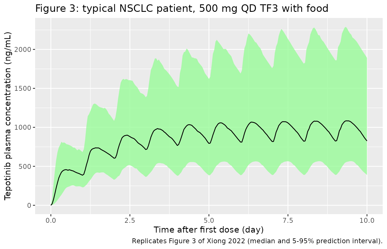
Values read off the published Figure 3 by the maintainers: median peak about 460 ng/mL on day 1 at about 0.5 day, median peak about 1110 ng/mL and median trough about 850 ng/mL over day 9-10, and a day-9 peak prediction interval of roughly 590-2050 ng/mL.
day1 <- fig3 |> filter(time <= 24)
day9 <- fig3 |> filter(time >= 216, time <= 240)
fig3_check <- tibble(
  quantity = c("Day-1 median peak", "Day-1 median tmax (h)", "Day-9 median peak",
               "Day-10 median trough", "Day-9 peak 5th percentile",
               "Day-9 peak 95th percentile"),
  figure_3 = c(460, 12, 1110, 850, 590, 2050),
  simulated = c(max(day1$Q50), day1$time[which.max(day1$Q50)], max(day9$Q50),
                tail(day9$Q50, 1), day9$Q05[which.max(day9$Q50)],
                day9$Q95[which.max(day9$Q50)])
) |>
  mutate(pct_diff = 100 * (simulated / figure_3 - 1))
knitr::kable(fig3_check, digits = 1,
caption = "Simulated versus digitised Figure 3 values.")| quantity | figure_3 | simulated | pct_diff |
|---|---|---|---|
| Day-1 median peak | 460 | 457.1 | -0.6 |
| Day-1 median tmax (h) | 12 | 11.0 | -8.3 |
| Day-9 median peak | 1110 | 1083.8 | -2.4 |
| Day-10 median trough | 850 | 825.7 | -2.9 |
| Day-9 peak 5th percentile | 590 | 552.5 | -6.4 |
| Day-9 peak 95th percentile | 2050 | 2289.5 | 11.7 |
# The medians are centre-of-distribution statistics of 200 subjects and move
# by a few percent between rxode2 builds; a 10% error in CL/F, F, the dose
# (e.g. 500 instead of 450 mg free base) or Vc moves them by more than 10%.
stopifnot(
  abs(fig3_check$pct_diff[c(1, 3, 4)]) < 12,
  # The tails of 200 subjects are noisier, so they get a wider envelope.
  abs(fig3_check$pct_diff[c(5, 6)]) < 30
)
The absorption rate constant: Table 3 versus ESM 13
Table 3 gives ka = 0.278 1/h; the ESM 13 equation sheet prints ka = 1.47 1/h. The two values give clearly different profile shapes, and Figure 3 decides between them: with ka = 1.47 1/h the day-1 peak arrives at about 5.5 h and the steady-state peak-to-trough ratio is about 1.6, whereas Figure 3 shows a broad day-1 peak at about half a day and a peak-to-trough ratio of about 1.3. The packaged model uses the Table 3 value.
ev_typ <- make_events(1, dose_label = 500, n_doses = 10,
                      obs_times = seq(0, 240, by = 0.25))
typ_table3 <- rxode2::rxSolve(mod, events = ev_typ, omega = NA, sigma = NA,
                              returnType = "data.frame")
mod_esm13 <- mod |> rxode2::ini(lka = log(1.47))
#> ℹ parameter labels from comments will be replaced by 'label()'
#> ℹ change initial estimate of `lka` to `0.385262400790645`
typ_esm13 <- rxode2::rxSolve(mod_esm13, events = ev_typ, omega = NA, sigma = NA,
                             returnType = "data.frame")

profile_shape <- function(sim) {
  d1 <- sim |> filter(time <= 24)
  d9 <- sim |> filter(time >= 216, time <= 240)
  c(tmax_day1 = d1$time[which.max(d1$Cc)],
    peak_trough_day9 = max(d9$Cc) / tail(d9$Cc, 1))
}
ka_shape <- rbind(`Table 3 (ka = 0.278)` = profile_shape(typ_table3),
                  `ESM 13 (ka = 1.47)` = profile_shape(typ_esm13),
                  `Figure 3 (digitised)` = c(12, 1110 / 850))
knitr::kable(ka_shape, digits = 2,
caption = "Typical-value profile shape under the two printed ka values.")| tmax_day1 | peak_trough_day9 | |
|---|---|---|
| Table 3 (ka = 0.278) | 11.50 | 1.38 |
| ESM 13 (ka = 1.47) | 5.75 | 1.64 |
| Figure 3 (digitised) | 12.00 | 1.31 |
stopifnot(
  abs(ka_shape[1, "tmax_day1"] - 12) < 2,
  abs(ka_shape[1, "peak_trough_day9"] - 1110 / 850) < 0.1,
  abs(ka_shape[2, "peak_trough_day9"] - 1110 / 850) > 0.2
)

bind_rows(
  typ_table3 |> mutate(source = "Table 3: ka = 0.278 1/h"),
  typ_esm13 |> mutate(source = "ESM 13: ka = 1.47 1/h")
) |>
  ggplot(aes(time / 24, Cc, colour = source)) +
  geom_line() +
  labs(x = "Time after first dose (day)", y = "Tepotinib (ng/mL)", colour = NULL,
       title = "Typical NSCLC patient, 500 mg QD TF3 with food") +
  theme(legend.position = "bottom")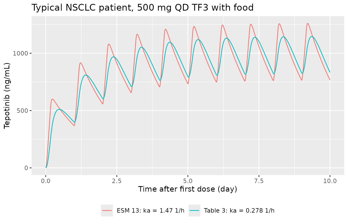
Replicate Figure 2: steady-state AUC versus dose
Figure 2 plots the predicted tepotinib AUC at steady state against dose for the typical NSCLC patient, with and without the dose effect on F. At steady state AUC = F x amt / CL, so the curve follows in closed form from the model’s own parameters. The model is also solved at 100, 500 and 1400 mg to confirm the closed form.
f_dose <- function(dose) 1 - 0.0412 / 100 * (dose - 500)
fig2 <- tibble(dose = seq(100, 1400, by = 10)) |>
  mutate(
    with_dose_effect = f_dose(dose) * 0.9 * dose / 20.4 * 1000,
    dose_independent = 0.9 * dose / 20.4 * 1000
  )

ggplot(fig2, aes(dose)) +
  geom_line(aes(y = with_dose_effect, linetype = "With the estimated dose effect on F"), colour = "blue") +
  geom_line(aes(y = dose_independent, linetype = "Assuming a dose-independent F"), colour = "grey40") +
  scale_linetype_manual(values = c("dashed", "solid")) +
  labs(x = "Dose (mg)", y = "Predicted tepotinib AUCss (ng*h/mL)", linetype = NULL,
       title = "Figure 2: AUCss versus dose (typical NSCLC patient, TF2 reference)",
       caption = "Replicates Figure 2 of Xiong 2022.") +
  theme(legend.position = "bottom")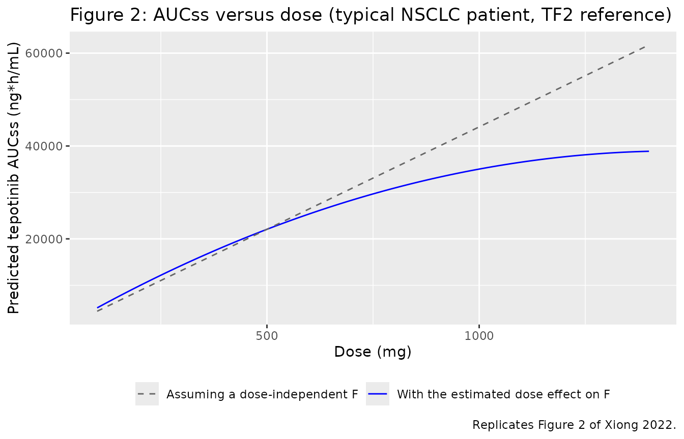
The figure’s AUCss of about 22,000 ngh/mL at 500 mg is reproduced with the reference formulation (TF2, F = 1); applying the TF3 effect (+15.4%) would give about 25,500 ngh/mL. The ESM 2 bootstrap AUCss at 500 mg (22,274 ngh/mL) and at 250 mg (12,277 ngh/mL) match the same TF2-reference values, so Figure 2 and ESM 2’s AUC rows evidently use F without the TF3 effect even though their captions mention TF3.
ev_auc <- bind_rows(lapply(seq_along(c(100, 250, 500, 1400)), function(i) {
  d <- c(100, 250, 500, 1400)[i]
  make_events(1, dose_label = d, n_doses = 90, obs_times = seq(2136, 2160, by = 0.25),
              tf3 = 0, id_offset = i - 1L, regimen = paste(d, "mg"))
}))
sim_auc <- rxode2::rxSolve(mod, events = ev_auc, omega = NA, sigma = NA,
                           keep = "regimen", returnType = "data.frame")
auc_check <- sim_auc |>
  group_by(regimen) |>
  summarise(auc_tau = sum(diff(time) * (head(Cc, -1) + tail(Cc, -1)) / 2), .groups = "drop") |>
  mutate(dose = as.numeric(sub(" mg", "", regimen)),
         closed_form = f_dose(dose) * 0.9 * dose / 20.4 * 1000,
         pct_diff = 100 * (auc_tau / closed_form - 1)) |>
  arrange(dose)
knitr::kable(auc_check, digits = 1,
caption = "Day-90 AUC over the dosing interval versus F x amt / CL.")| regimen | auc_tau | dose | closed_form | pct_diff |
|---|---|---|---|---|
| 100 mg | 5103.5 | 100 | 5138.8 | -0.7 |
| 250 mg | 12081.9 | 250 | 12165.4 | -0.7 |
| 500 mg | 21907.4 | 500 | 22058.8 | -0.7 |
| 1400 mg | 38595.6 | 1400 | 38862.4 | -0.7 |
stopifnot(
  # 90 days approaches but does not quite reach steady state through the slow
  # peripheral compartment (k21 = Q/Vp = 0.0011 1/h); the residual shortfall
  # is about 1%.
  all(abs(auc_check$pct_diff) < 3),
  # Figure 2 read-offs: ~22,000 at 500 mg and ~39,000 at 1400 mg.
  abs(auc_check$closed_form[auc_check$dose == 500] / 22000 - 1) < 0.05,
  abs(auc_check$closed_form[auc_check$dose == 1400] / 39000 - 1) < 0.05,
  # Results: 'relative bioavailability for the supratherapeutic tepotinib dose
  # of 1000 mg is 0.79 compared with the Fpar for a dose of 500 mg'.
  abs(f_dose(1000) - 0.79) < 0.01
)
Clearance versus eGFR (Results)
The Results give typical CL/F values of 16.2, 18.6, 19.7 and 20.9 L/h at eGFR values of 30, 60, 80 and 110 mL/min/1.73 m^2 for a typical individual receiving 500 mg.
egfr_check <- tibble(
  eGFR = c(30, 60, 80, 110),
  published = c(16.2, 18.6, 19.7, 20.9),
  model = 20.4 * (eGFR / 97.28)^0.199
)
knitr::kable(egfr_check, digits = 2, caption = "CL/F (L/h) versus eGFR.")| eGFR | published | model |
|---|---|---|
| 30 | 16.2 | 16.14 |
| 60 | 18.6 | 18.53 |
| 80 | 19.7 | 19.62 |
| 110 | 20.9 | 20.91 |
PKNCA validation against ESM 2
ESM 2 tabulates bootstrap steady-state exposures for cancer patients at 500 mg and 250 mg once daily, with food, and an effective half-life of 32.1 h (the main text quotes about 32 h). The typical NSCLC patient taking TF3 with food is simulated for 90 days, and steady-state Cmax, Ctrough and AUC0-24 come from PKNCA over the last dosing interval.
ev_ss <- bind_rows(
  make_events(1, dose_label = 500, n_doses = 90, obs_times = seq(2136, 2160, by = 0.25),
              id_offset = 0L, regimen = "500 mg QD"),
  make_events(1, dose_label = 250, n_doses = 90, obs_times = seq(2136, 2160, by = 0.25),
              id_offset = 1L, regimen = "250 mg QD")
)
stopifnot(!anyDuplicated(unique(ev_ss[, c("id", "time", "evid")])))
sim_ss <- rxode2::rxSolve(mod, events = ev_ss, omega = NA, sigma = NA,
                          keep = "regimen", returnType = "data.frame")

conc_ss <- sim_ss |>
  filter(!is.na(Cc)) |>
  select(id, time, Cc, regimen)
dose_ss <- ev_ss |>
  filter(evid == 1, time == 2136) |>
  select(id, time, amt, regimen)

conc_obj <- PKNCA::PKNCAconc(conc_ss, Cc ~ time | regimen + id)
dose_obj <- PKNCA::PKNCAdose(dose_ss, amt ~ time | regimen + id)
intervals <- data.frame(start = 2136, end = 2160, cmax = TRUE, cmin = TRUE,
                        auclast = TRUE)
nca_res <- PKNCA::pk.nca(PKNCA::PKNCAdata(conc_obj, dose_obj, intervals = intervals))

published <- tibble::tribble(
  ~regimen,    ~cmax, ~cmin, ~auclast,
  "500 mg QD", 1236,  952,   22274,
  "250 mg QD", 683,   523,   12277
)
cmp <- nlmixr2lib::ncaComparisonTable(
  simulated = nca_res,
  reference = published,
  by = "regimen",
  units = c(cmax = "ng/mL", cmin = "ng/mL", auclast = "ng*h/mL"),
  tolerance_pct = 20
)
knitr::kable(cmp, caption = "Simulated typical NSCLC patient (TF3, fed) versus ESM 2 bootstrap means. * differs by >20%.")| NCA parameter | regimen | Reference | Simulated | % diff |
|---|---|---|---|---|
| Cmax (ng/mL) | 500 mg QD | 1240 | 1200 | -3.3% |
| Cmax (ng/mL) | 250 mg QD | 683 | 659 | -3.5% |
| Cmin (ng/mL) | 500 mg QD | 952 | 874 | -8.2% |
| Cmin (ng/mL) | 250 mg QD | 523 | 482 | -7.8% |
| AUClast (ng*h/mL) | 500 mg QD | 22300 | 25300 | +13.5% |
| AUClast (ng*h/mL) | 250 mg QD | 12300 | 13900 | +13.6% |
No row differs by more than 20%. The simulated AUC0-24 is about 14% above ESM 2 because ESM 2’s AUC rows correspond to the TF2-reference F (see the Figure 2 section), while its Cmax and Ctrough agree with TF3 to within 10%. ESM 2 is not internally consistent on this point: its 500 mg AUCss implies an average concentration of 928 ng/mL, below its own mean Ctrough of 952 ng/mL, which no single concentration profile can produce.
sim_vals <- as.data.frame(nca_res) |>
  filter(PPTESTCD %in% c("cmax", "cmin", "auclast")) |>
  select(regimen, PPTESTCD, PPORRES) |>
  tidyr::pivot_wider(names_from = PPTESTCD, values_from = PPORRES) |>
  left_join(published, by = "regimen", suffix = c("_sim", "_pub"))
stopifnot(
  all(abs(sim_vals$cmax_sim / sim_vals$cmax_pub - 1) < 0.1),
  all(abs(sim_vals$cmin_sim / sim_vals$cmin_pub - 1) < 0.15),
  all(abs(sim_vals$auclast_sim / sim_vals$auclast_pub - 1) < 0.2)
)
Effective half-life
The effective half-life follows from an accumulation ratio R (steady state over first dose) as t1/2,eff = tau x ln 2 / ln(R / (R - 1)); it does not depend on F or the dose. ESM 2 reports 32.1 h (bootstrap 5th-95th percentile 31.4-32.9 h) and the text “~32 h”, but neither says which accumulation ratio was used. For a two-compartment drug the choice matters, so all three common versions are shown.
ev_acc <- make_events(1, dose_label = 500, n_doses = 90,
                      obs_times = c(seq(0, 24, by = 0.25), seq(2136, 2160, by = 0.25)))
sim_acc <- rxode2::rxSolve(mod, events = ev_acc, omega = NA, sigma = NA,
                           returnType = "data.frame")
auc_window <- function(d, a, b) {
  w <- d |> filter(time >= a, time <= b)
  sum(diff(w$time) * (head(w$Cc, -1) + tail(w$Cc, -1)) / 2)
}
t_eff <- function(R) 24 * log(2) / log(R / (R - 1))
day1 <- sim_acc |> filter(time <= 24)
day90 <- sim_acc |> filter(time >= 2136)
R_acc <- c(
  AUC0_24 = auc_window(sim_acc, 2136, 2160) / auc_window(sim_acc, 0, 24),
  Cmax = max(day90$Cc) / max(day1$Cc),
  Ctrough = tail(day90$Cc, 1) / tail(day1$Cc, 1)
)
t_half_eff <- tibble(ratio_basis = names(R_acc), R = R_acc, t_half_eff_h = t_eff(R_acc))
knitr::kable(t_half_eff, digits = 2,
caption = "Typical NSCLC patient: effective half-life by accumulation-ratio basis (ESM 2: 32.1 h).")| ratio_basis | R | t_half_eff_h |
|---|---|---|
| AUC0_24 | 2.67 | 35.49 |
| Cmax | 2.34 | 29.85 |
| Ctrough | 2.21 | 27.53 |
# Known deviation: the AUC-based value is about 35.5 h, 11% above ESM 2's
# 32.1 h; the Cmax- and Ctrough-based values (about 30 h and 27.5 h) fall
# below it, so the published value lies inside the range of estimators.
# The estimator behind 32.1 h is not stated and ESM 2 averages over the
# covariates of the cancer patients, so the gap is recorded rather than
# chased. The envelope still breaks on a mis-transcribed CL/F, Vc/F or Q/F.
stopifnot(
  abs(t_half_eff$t_half_eff_h[t_half_eff$ratio_basis == "AUC0_24"] / 32.1 - 1) < 0.15,
  min(t_half_eff$t_half_eff_h) < 32.1, max(t_half_eff$t_half_eff_h) > 32.1
)
MSC2571109A
The metabolite model has no published exposure summary to compare against (ESM 11 is a forest plot of relative AUC), so its typical profile is shown for the same regimen. Because the fraction metabolised is fixed to 1, the metabolite amounts are expressed as parent-equivalent mass; the predicted concentrations are unaffected by that choice (Discussion).
typ_table3 |>
  select(time, Tepotinib = Cc, MSC2571109A = Cc_msc2571109a) |>
  tidyr::pivot_longer(-time, names_to = "analyte", values_to = "conc") |>
  ggplot(aes(time / 24, conc, colour = analyte)) +
  geom_line() +
  labs(x = "Time after first dose (day)", y = "Plasma concentration (ng/mL)",
       colour = NULL, title = "Typical NSCLC patient, 500 mg QD TF3 with food") +
  theme(legend.position = "bottom")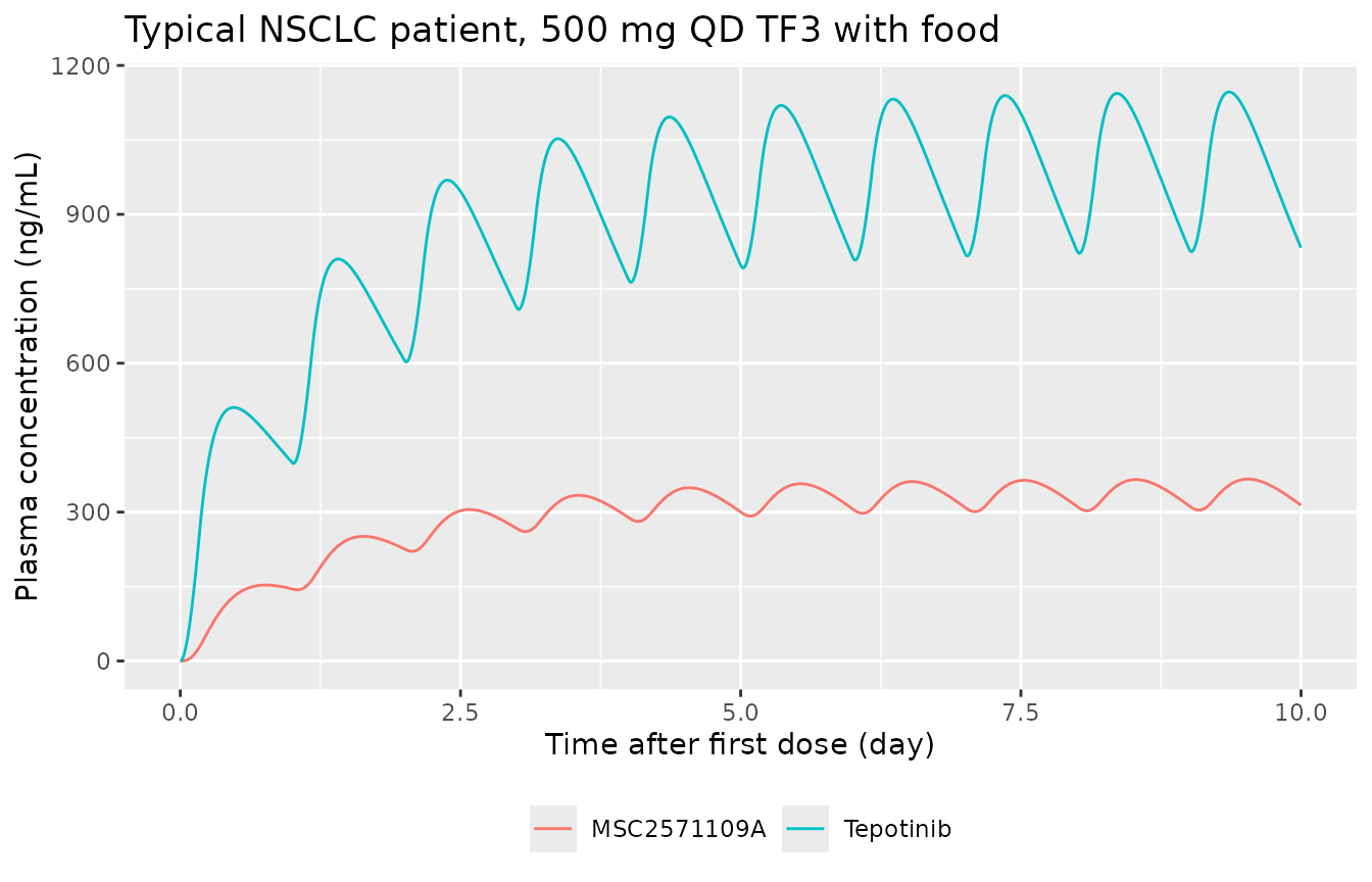
Assumptions and deviations
- ka. Table 3 (0.278 1/h) and the ESM 13 equation sheet (1.47 1/h) disagree. The Table 3 value is used because only it reproduces the profile shape of Figure 3 (see the ka check above).
- Vc/F. Table 3 prints 1020 L and ESM 13 prints 1030 L. The 1% difference cannot be resolved from the figures; the Table 3 value is used because Table 3 is the parameter-estimate table and ESM 13 is demonstrably unreliable on ka.
-
Salt-to-base factor. The tabulated apparent
parameters apply to the free-base amount (Table 3 footnote a), so
amtis 0.9 x the labelled dose, while theDOSEcovariate is the labelled dose used by the ESM 13 dose effect on F. - IIV scale. The Methods define IIV as log-normal “with standard deviation omega”, and Table 3 reports each IIV next to “(CV)”. The tabulated number is read as omega, so each variance is the value squared (for example CL/F 0.335^2 = 0.1122). Reading it as a true CV, omega^2 = log(1 + CV^2), would give 0.1061 for CL/F and, for the widest terms, 0.355 instead of 0.426 (ka) and 0.505 instead of 0.738 (Vc,met). The Figure 3 prediction interval cannot separate the two readings.
- Subgroup-specific IIV. Table 3 reports separate IIV magnitudes for CL/F and F in healthy participants, for F on CF1 doses, and for metabolite CL in healthy participants. The control stream is not published, so the scoping is reconstructed as mutually exclusive etas: healthy participants draw the healthy-participant eta; patients draw the CF1 eta on CF1 dose records and the patient eta otherwise (CF1 was used only in patients, in study 001).
-
IIV on the fraction metabolised. The Results state
that IIV on FM was estimated, but Table 3 does not report its value. It
is carried as
etalfm ~ fixed(0), so stochastic simulations understate metabolite between-subject variability. - No correlations between etas are reported, so the omega matrix is diagonal.
- Residual error. The paper used an additive error on log-transformed concentrations; it is encoded as the equivalent proportional error in linear space, with the tabulated SDs 0.337 (tepotinib) and 0.298 (MSC2571109A).
-
Metabolite covariate forms. ESM 13 covers only the
parent. The metabolite covariates follow the Methods’ Formula 1 (power,
normalised to the reference participant’s eGFR 97.28 and weight 72 kg)
and Formula 2 (
1 + thetafor an indicator); “Patient/participant covariate on Vp,met” is applied to healthy participants, as ESM 13 does for the parent’s Vp. -
East Asian. The metabolite “East Asian” covariate
pools the paper’s Japanese and Other East Asian categories and is mapped
to
RACE_ASIAN_NORTHEAST. - Serum albumin reference. The Table 3 footnote’s “4 g/L” is read as 40 g/L, as in ESM 13 and the Figure 2 and 3 captions.
- Figure 2 and ESM 2 formulation. Both captions describe TF3 with food, but their AUC values match the reference formulation TF2 (F = 1); see the Figure 2 and PKNCA sections.
- Effective half-life. The model’s AUC-accumulation effective half-life for the typical NSCLC patient is about 35.5 h, 11% above the 32.1 h of ESM 2; the paper does not state its estimator, and the Cmax- and Ctrough-based versions (about 30 h and 27.5 h) fall below it, so 32.1 h lies inside the range of the three estimators.
- Figures 4 and 5 (AUCss by race and the covariate forest plot) are built from the individual covariates of the analysis data set, which are not public, and are not replicated.
- No erratum or correction notice is linked to this article in Europe PMC as of 2026-10-01.