Nivolumab triple-negative breast cancer QSP (Ruiz-Martinez 2022)
Source:vignettes/articles/RuizMartinez_2022_nivolumab_qsp.Rmd
RuizMartinez_2022_nivolumab_qsp.Rmd
# Build once and reuse: this is a 120-state model, and every build costs
# several seconds.
mod <- rxode2::rxode2(readModelDb("RuizMartinez_2022_nivolumab_qsp"))
Model and source
- Citation: Ruiz-Martinez A, Gong C, Wang H, Sove RJ, Mi H, Kimko H, Popel AS. Simulations of tumor growth and response to immunotherapy by coupling a spatial agent-based model with a whole-patient quantitative systems pharmacology model. PLoS Comput Biol. 2022;18(7):e1010254. doi:10.1371/journal.pcbi.1010254.
- Article: https://doi.org/10.1371/journal.pcbi.1010254
- Code and SBML deposit: https://github.com/popellab/SPQSP_IO_TNBC
Ruiz-Martinez et al. couple a whole-patient quantitative systems pharmacology (QSP) model of triple-negative breast cancer (TNBC) to a stochastic, spatial agent-based model (ABM) of the tumour, giving a “spatial QSP” (spQSP) model. The ABM replaces the QSP tumour compartment: it carries cancer stem-like, progenitor and senescent cells and individual T cells and MDSCs on a 3-D voxel grid, recruits immune cells from the QSP blood compartment at random entry points, and hands the cell counts back to the QSP model every time step.
Only the QSP layer is packaged here. The ABM is a stochastic, rule-based simulation on a spatial grid and cannot be written as ODEs; it is documented in the paper and in the authors’ C++ code.
The QSP layer is the Wang 2020 HER2-negative breast-cancer model
(Wang_2020_entinostat_nivolumab_ipilimumab_qsp) with its
equations unchanged (“Without modifying the differential and algebraic
equations from Wang et al. [46] model, we have recalibrated some
parameters”), recalibrated so that the virtual patients reproduce the
anti-PD-1 responder numbers and the tumour T cell densities of TNBC. The
authors list the full model in S1 Table (compartments, parameters with
their sampling ranges, the 154 reactions, the rules, the 120 species and
the single event) and the parameter set used for every simulation of the
paper in S2 Table (sheet “QSP default parameters”, with per-figure
overrides on the later sheets). The SBML file in the code deposit is the
Wang 2020 SBML with four of those parameters updated; its reactions,
rules, species and event are identical to Wang 2020.
The packaged model is therefore the Wang 2020 translation (amount-based states, a single consistent unit system, dimension-checked rate laws; see that model’s article for the translation details) carrying the S2 Table default parameter values. Thirty-seven parameters differ from Wang 2020; they are tabulated below.
Model outputs: tumour_diameter (cm, from the total
tumour volume assuming a sphere), Cc_nivolumab (central
nivolumab concentration, nmol/L) and the tumour-infiltrating cell
densities teff_density, treg_density,
mdsc_density (cells per mL of tumour). Cell counts are read
directly from the states, for example q_V_T_C1 (cancer
cells), q_V_C_T1 / q_V_C_T0 (effector /
regulatory T cells in blood) and q_V_T_T1,
q_V_T_T_exh, q_V_T_T0 (effector, exhausted and
regulatory T cells in the tumour). Nivolumab is dosed in nmol into
q_V_C_nivo.
There are no etas and no residual-error model: the authors generated virtual patients by sampling the parameter ranges of S1 Table, not by fitting inter-individual variability.
Population
This is a methodological in silico study; no clinical data were
fitted directly. The QSP parameters were recalibrated against the
responder numbers and tumour T cell densities of the phase 1 entinostat
+ nivolumab trial ETCTN-9844 (Torres 2021, the paper’s reference 51),
and S1 and S2 Figs show 100 virtual TNBC patients sampled from the S1
Table ranges, without and with nivolumab 3 mg/kg every 2 weeks. Each
simulation starts from a single cancer cell; therapy starts when the
tumour reaches its pre-treatment diameter
(initial_tumour_diameter, 2.255 cm in the default set). S2
Table sizes the nivolumab dose for an 80 kg patient with a molecular
weight of 144.6 kDa.
Source trace
| Model element | Source |
|---|---|
Model structure: 154 reaction rates
v1-v154, 21 repeated-assignment rules, 120
species and their initial amounts, cancer-cell elimination event |
S1 Table, sheets “Table S3. Reactions”, “Table S4. Rules”, “Table S5. Species”, “Table S6.Events”; identical to the Wang 2020 SBML (checked below) |
8 compartment capacities (vol_*) |
S1 Table, sheet “Table S1. Compartment” |
| 187 model parameters | S2 Table, sheet “QSP default parameters” (value and unit in each line’s comment), with the S1 Table sampling range noted where one is printed |
Growth-rate cases (slow / medium / fast: k_C1_growth,
k_C_T1, k_T1, Treg_max) |
Table 4; S2 Table, sheet “Figures 7 & 8” |
| Nivolumab regimen, body weight 80 kg, molecular weight 144.6 kDa | Results, “Spatial distribution of cell densities with immunotherapy”; S2 Table, sheets “Figures 4 & 5” and “Figures 7 & 8” |
Pre-treatment diameter 2.255 cm
(initial_tumour_diameter) |
S2 Table, sheet “QSP default parameters” |
| Untreated blood T cell trajectories used for the qualitative check | Figure 6A (digitised by the maintainers) |
F_ENT_buccal = 0.324 (entinostat route split) |
Not in this paper; carried from
Wang_2020_entinostat_nivolumab_ipilimumab_qsp. Entinostat
is not dosed here. |
Simulation set-up
# Dosing conversion for the vignette (not model parameters): S2 Table.
wt_kg <- 80
mw_nivo <- 144600 # g/mol
nivo_nmol <- 3 * wt_kg / mw_nivo * 1e6
d0 <- readModelDb("RuizMartinez_2022_nivolumab_qsp")
ini_df <- rxode2::rxode2(d0)$iniDf
diam0 <- 2.255 # cm, S2 Table initial_tumour_diameter

# method = "cvode" (SUNDIALS BDF), as for Wang 2020: lsoda sits on a numerical
# knife-edge for this model family.
SOLVE <- function(m, ev, params = NULL) {
  rxode2::rxSolve(m, ev, params = params, method = "cvode", maxsteps = 1e6, returnType = "data.frame")
}

# First time a monotonically growing output reaches `level`, interpolated
# linearly between the bracketing grid points.
first_crossing <- function(time, y, level) {
  i <- which(y >= level)[1]
  time[i - 1] + (level - y[i - 1]) / (y[i] - y[i - 1]) * (time[i] - time[i - 1])
}

# Grow from one cancer cell, find the time the diameter reaches `diam`, then
# solve untreated and nivolumab arms from that time for `days`.
run_case <- function(params = NULL, diam = diam0, days = 360) {
  g <- SOLVE(mod, rxode2::et(seq(0, 8000, by = 5)), params = params)
  ts <- first_crossing(g$time, g$tumour_diameter, diam)
  obs <- c(seq(0, ts, length.out = 200), ts + seq(0, days, by = 2))
  untreated <- SOLVE(mod, rxode2::et(obs), params = params)
  treated <- SOLVE(
    mod,
    rxode2::et(obs) |>
      rxode2::et(time = ts, amt = nivo_nmol, cmt = "q_V_C_nivo", ii = 14, addl = floor(days / 14)),
    params = params
  )
  bind_rows(
    mutate(untreated, arm = "Untreated"),
    mutate(treated, arm = "Nivolumab 3 mg/kg q2w")
  ) |>
    mutate(t_start = ts, day = time - ts)
}
The model equations are Wang 2020’s
The structure is checked rather than assumed: setting the 37 recalibrated parameters back to their Wang 2020 values must reproduce the packaged Wang 2020 model exactly. Both models use the same ODEs, so the difference is pure numerical error and the bound is tight.
wang <- rxode2::rxode2(readModelDb("Wang_2020_entinostat_nivolumab_ipilimumab_qsp"))
p_rm <- setNames(ini_df$est, ini_df$name)
p_wang <- setNames(wang$iniDf$est, wang$iniDf$name)
stopifnot(setequal(names(p_rm), names(p_wang)))
p_wang <- p_wang[names(p_rm)]
changed <- names(p_rm)[abs(p_rm - p_wang) > 1e-9 * pmax(abs(p_rm), abs(p_wang))]
length(changed)
#> [1] 37

grid_id <- rxode2::et(seq(0, 5000, by = 25))
s_wang <- SOLVE(wang, grid_id)
s_back <- SOLVE(mod, grid_id, params = p_wang[changed])
rel <- function(a, b) max(abs(a - b) / pmax(abs(b), 1e-6))
c(
  diameter = rel(s_back$tumour_diameter, s_wang$tumour_diameter),
  cancer = rel(s_back$q_V_T_C1, s_wang$q_V_T_C1),
  teff_blood = rel(s_back$q_V_C_T1, s_wang$q_V_C_T1),
  treg_tumour = rel(s_back$q_V_T_T0, s_wang$q_V_T_T0)
)
#>    diameter      cancer  teff_blood treg_tumour
#>           0           0           0           0
stopifnot(
  length(changed) == 37,
  rel(s_back$tumour_diameter, s_wang$tumour_diameter) < 1e-5,
  rel(s_back$q_V_T_C1, s_wang$q_V_T_C1) < 1e-5,
  rel(s_back$q_V_C_T1, s_wang$q_V_C_T1) < 1e-5,
  rel(s_back$q_V_T_T0, s_wang$q_V_T_T0) < 1e-5
)
The recalibrated parameters (values in the model unit system: counts, litres, days):
data.frame(
  parameter = changed,
  wang = unname(p_wang[changed]),
  rm = unname(p_rm[changed])
) |>
  mutate(ratio = rm / wang, across(c(wang, rm, ratio), \(x) signif(x, 4))) |>
  dplyr::rename(
    "Parameter" = parameter, "Wang 2020" = wang,
    "Ruiz-Martinez 2022" = rm, "Ratio" = ratio
  ) |>
knitr::kable(caption = "Parameters recalibrated by Ruiz-Martinez 2022 (S2 Table) relative to Wang 2020.")| Parameter | Wang 2020 | Ruiz-Martinez 2022 | Ratio |
|---|---|---|---|
| k_C1_growth | 6.730e-03 | 5.000e-03 | 0.7429 |
| k_C1_death | 1.000e-04 | 3.000e-05 | 0.3000 |
| q_T0_P_out | 1.500e-02 | 2.400e+01 | 1600.0000 |
| q_T0_T_in | 4.824e+00 | 1.440e+01 | 2.9850 |
| N0 | 2.000e+00 | 5.000e+00 | 2.5000 |
| N_costim | 3.000e+00 | 6.000e+00 | 2.0000 |
| N_IL2 | 1.100e+01 | 1.400e+01 | 1.2730 |
| k_Treg | 1.000e+00 | 2.440e-01 | 0.2440 |
| n_T1_clones | 1.000e+02 | 6.136e+01 | 0.6136 |
| q_T1_P_out | 1.000e+00 | 2.400e+01 | 24.0000 |
| q_T1_T_in | 4.824e+00 | 1.440e+01 | 2.9850 |
| k_T1 | 1.000e-01 | 1.340e-01 | 1.3400 |
| k_C_T1 | 2.000e+00 | 7.360e-01 | 0.3680 |
| k_P1_d1 | 2.409e+16 | 3.342e+16 | 1.3880 |
| CD28_CD8X_50 | 2.000e+12 | 1.700e+13 | 8.5020 |
| C1_PDL1_total | 1.600e+06 | 3.872e+05 | 0.2420 |
| C1_PDL2_total | 2.000e+03 | 4.000e+04 | 20.0000 |
| Treg_CTLA4_50 | 1.000e+03 | 6.171e+02 | 0.6171 |
| k_CTLA4_ADCC | 1.000e-01 | 2.890e-01 | 2.8900 |
| IC50_ENT_C | 2.252e+17 | 4.343e+16 | 0.1928 |
| k_sec_CCL2 | 8.551e+04 | 8.144e+04 | 0.9523 |
| k_sec_NO | 2.891e+08 | 2.405e+08 | 0.8321 |
| k_sec_ArgI | 8.431e+15 | 7.904e+15 | 0.9375 |
| IC50_ENT_NO | 3.372e+14 | 1.131e+15 | 3.3530 |
| ki_Treg | 2.700e+00 | 1.402e+00 | 0.5193 |
| IC50_ArgI_CTL | 3.716e+25 | 2.055e+26 | 5.5300 |
| IC50_NO_CTL | 4.517e+14 | 1.619e+15 | 3.5840 |
| EC50_ArgI_Treg | 1.331e+25 | 2.853e+25 | 2.1440 |
| MDSC_max | 1.637e+08 | 1.664e+08 | 1.0170 |
| Treg_max | 9.550e+05 | 9.000e+08 | 942.4000 |
| IC50_ENT_CCL2 | 7.227e+14 | 9.815e+14 | 1.3580 |
| IC50_ENT_ArgI | 3.011e+17 | 2.252e+17 | 0.7480 |
| k_a1_ENT | 4.560e+01 | 5.033e+01 | 1.1040 |
| k_a2_ENT | 5.928e+01 | 1.230e+02 | 2.0750 |
| k_cln_ENT | 1.766e+21 | 1.337e+21 | 0.7568 |
| q_T_ENT | 2.765e+05 | 2.861e+05 | 1.0350 |
| k_cl_ENT | 3.648e+00 | 1.450e+01 | 3.9750 |
The largest structural shifts are faster T cell egress from the
peripheral compartment (q_T0_P_out,
q_T1_P_out), three-fold faster T cell entry into the tumour
(q_T0_T_in, q_T1_T_in), more T cell
generations per activation (N0, N_costim,
N_IL2), a much higher maximal Treg density in the tumour
(Treg_max), lower PD-L1 expression on cancer cells
(C1_PDL1_total) and a lower cancer-cell killing rate by T
cells (k_C_T1). The entinostat parameters also changed, but
entinostat is not dosed in this paper.
Growth-rate cases of Table 4
Table 4 prints its growth-rate cases as ratios; the per-case values in S2 Table must reproduce them.
k_treg <- p_rm[["k_Treg"]]
cases <- data.frame(
  case = c("Slow", "Medium", "Fast"),
  k_C1_growth = c(0.005, 0.01, 0.015),
  k_C_T1 = c(0.7, 1.4, 1.4),
  k_T1 = c(0.134, 0.27, 0.27),
  Treg_max = c(9e5, 2e6, 2e6) # cells/mL
)
cases <- mutate(cases, growth_kill = k_C1_growth / k_C_T1, t1_treg = k_T1 / k_treg)
cases |>
  dplyr::rename(
    "Case" = case, "k_C1,growth (1/day)" = k_C1_growth, "k_C,T1 (1/day)" = k_C_T1,
    "k_T1 (1/day)" = k_T1, "Treg,max (cells/mL)" = Treg_max,
    "k_C1,growth / k_C,T1" = growth_kill, "k_T1 / k_Treg" = t1_treg
  ) |>
knitr::kable(digits = 4, caption = "S2 Table per-case values and the ratios they imply; Table 4 prints 7e-3 / 7e-3 / 1.1e-2 and 0.56 / 1.12 / 1.12.")| Case | k_C1,growth (1/day) | k_C,T1 (1/day) | k_T1 (1/day) | Treg,max (cells/mL) | k_C1,growth / k_C,T1 | k_T1 / k_Treg |
|---|---|---|---|---|---|---|
| Slow | 0.005 | 0.7 | 0.134 | 9e+05 | 0.0071 | 0.5492 |
| Medium | 0.010 | 1.4 | 0.270 | 2e+06 | 0.0071 | 1.1066 |
| Fast | 0.015 | 1.4 | 0.270 | 2e+06 | 0.0107 | 1.1066 |
stopifnot(
  all(abs(cases$growth_kill / c(7e-3, 7e-3, 1.1e-2) - 1) < 0.05),
  all(abs(cases$t1_treg / c(0.56, 1.12, 1.12) - 1) < 0.03)
)
The slow-growth case is the S2 Table default except for
k_C_T1 (0.7 in the case table, 0.736 in the default
sheet).
Default virtual patient
def <- run_case()
t_start <- def$t_start[1]
t_start
#> [1] 4340.207
With the default parameters the tumour takes 4340 days (11.9 years) to grow from one cancer cell to the 2.255 cm pre-treatment diameter, the consequence of the slow growth rate of 0.005/day.
def_long <- def |>
  filter(day >= 0) |>
  transmute(
    arm, day,
    "Cancer cells" = q_V_T_C1,
    "Teff in blood" = q_V_C_T1,
    "Treg in blood" = q_V_C_T0,
    "Teff in tumour" = q_V_T_T1,
    "Treg in tumour" = q_V_T_T0,
    "MDSC in tumour" = q_V_T_MDSC
  ) |>
  pivot_longer(-c(arm, day), names_to = "quantity", values_to = "cells") |>
  filter(cells > 1e-1)
ggplot(def_long, aes(day, cells, colour = arm)) +
  geom_line(linewidth = 0.8) +
  facet_wrap(~quantity, scales = "free_y", ncol = 2) +
  scale_y_log10() +
  labs(x = "Days from the pre-treatment diameter", y = "Cells", colour = NULL) +
  theme_bw() +
  theme(legend.position = "bottom")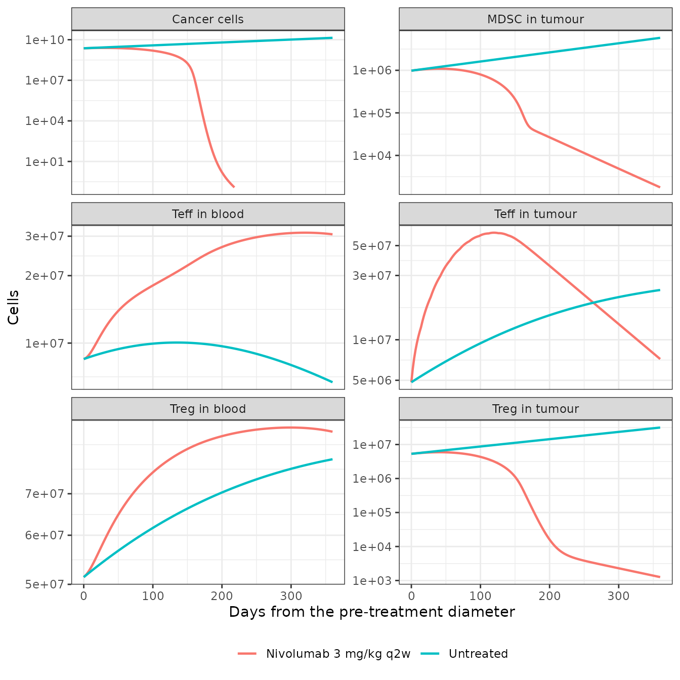
Default virtual patient from the pre-treatment diameter (day 0), untreated and under nivolumab 3 mg/kg every 2 weeks. Compare the per-patient panels of S1 Fig (untreated) and S2 Fig (nivolumab).
def_sum <- def |>
  filter(day >= 0) |>
  group_by(arm) |>
  summarise(
    c1_0 = q_V_T_C1[which.min(abs(day))],
    c1_180 = q_V_T_C1[which.min(abs(day - 180))],
    c1_360 = q_V_T_C1[which.min(abs(day - 360))],
    diam_180 = tumour_diameter[which.min(abs(day - 180))],
    teff_blood_peak = max(q_V_C_T1),
    .groups = "drop"
  )
def_sum |>
  dplyr::rename(
    "Arm" = arm, "Cancer cells, day 0" = c1_0, "Cancer cells, day 180" = c1_180,
    "Cancer cells, day 360" = c1_360, "Diameter, day 180 (cm)" = diam_180,
    "Peak Teff in blood" = teff_blood_peak
  ) |>
knitr::kable(digits = 3, format.args = list(scientific = 3), caption = "Default virtual patient.")| Arm | Cancer cells, day 0 | Cancer cells, day 180 | Cancer cells, day 360 | Diameter, day 180 (cm) | Peak Teff in blood |
|---|---|---|---|---|---|
| Nivolumab 3 mg/kg q2w | 2329393604 | 649.361 | 0 | 0.547 | 31098890 |
| Untreated | 2329393604 | 5677119500.502 | 13758943071 | 3.034 | 10055575 |
The default parameter set is a responder: under nivolumab the cancer cells are eliminated within a year, while the untreated tumour keeps growing. Its pre-treatment state lies inside the envelope of the 100 virtual patients of S1 Fig (cancer cells about 1e8-1e10, regulatory T cells in blood about 1e7-1e8, MDSCs in tumour about 1e4-1e8 at the start of the plotted window).
u <- def_sum[def_sum$arm == "Untreated", ]
n <- def_sum[def_sum$arm == "Nivolumab 3 mg/kg q2w", ]
stopifnot(
  # pre-treatment cancer cells within the S1 Fig envelope
  u$c1_0 > 1e8, u$c1_0 < 1e10,
  # untreated tumour grows over the year
  u$c1_360 > 3 * u$c1_0,
  # PD-1 blockade expands effector T cells in blood (Figure 6A, thin lines)
  n$teff_blood_peak > 1.5 * u$teff_blood_peak,
  # the default patient responds
  n$diam_180 < 0.5 * u$diam_180
)
Blood T cell trajectories against Figure 6A
Figure 6A plots the spQSP outputs for four ABM configurations. The blood compartment is a QSP compartment in the spQSP model as well (the ABM only replaces the tumour), so the untreated blood T cell trajectories are a qualitative check on the recalibrated QSP. The authors note that QSP and spQSP outcomes “are qualitatively equivalent but not exactly the same” (S1 Supplementary Material, section A.4), and the time axis of Figure 6 is the ABM’s own. The maintainers digitised the untreated (thick) lines, which almost coincide across the four cases, and aligned them to the QSP solution at the peak of the effector T cells in blood.
fig6 <- data.frame(
  quantity = c(rep("Teff in blood", 3), rep("Treg in blood", 2)),
  fig6_day = c(500, 790, 1000, 500, 1000),
  published = c(7.6e6, 1.27e7, 1.0e7, 6.4e7, 9.2e7)
)
grow <- SOLVE(mod, rxode2::et(seq(3000, 6000, by = 2)))
t_peak <- grow$time[which.max(grow$q_V_C_T1)]
fig6 <- fig6 |>
  mutate(
    time = t_peak + fig6_day - 790,
    simulated = ifelse(
      quantity == "Teff in blood",
      approx(grow$time, grow$q_V_C_T1, time)$y,
      approx(grow$time, grow$q_V_C_T0, time)$y
    ),
    ratio = simulated / published
  )
fig6 |>
  select(quantity, fig6_day, published, simulated, ratio) |>
  dplyr::rename(
    "Quantity" = quantity, "Figure 6 day" = fig6_day, "Figure 6A (digitised)" = published,
    "Packaged QSP" = simulated, "Ratio" = ratio
  ) |>
knitr::kable(digits = 2, format.args = list(scientific = 3), caption = "Untreated blood T cells: Figure 6A (spQSP) vs the packaged QSP, aligned at the effector T cell peak.")| Quantity | Figure 6 day | Figure 6A (digitised) | Packaged QSP | Ratio |
|---|---|---|---|---|
| Teff in blood | 500 | 7600000 | 4743177 | 0.62 |
| Teff in blood | 790 | 12700000 | 10055712 | 0.79 |
| Teff in blood | 1000 | 10000000 | 6994963 | 0.70 |
| Treg in blood | 500 | 64000000 | 35232549 | 0.55 |
| Treg in blood | 1000 | 92000000 | 78981977 | 0.86 |
traj <- grow |>
  transmute(fig6_day = time - t_peak + 790, "Teff in blood" = q_V_C_T1, "Treg in blood" = q_V_C_T0) |>
  filter(fig6_day >= 450, fig6_day <= 1050) |>
  pivot_longer(-fig6_day, names_to = "quantity", values_to = "cells")
ggplot(traj, aes(fig6_day, cells)) +
  geom_line() +
  geom_point(data = fig6, aes(y = published), colour = "red", size = 2) +
  facet_wrap(~quantity, scales = "free_y") +
  labs(x = "Figure 6 time axis (days)", y = "Cells") +
  theme_bw()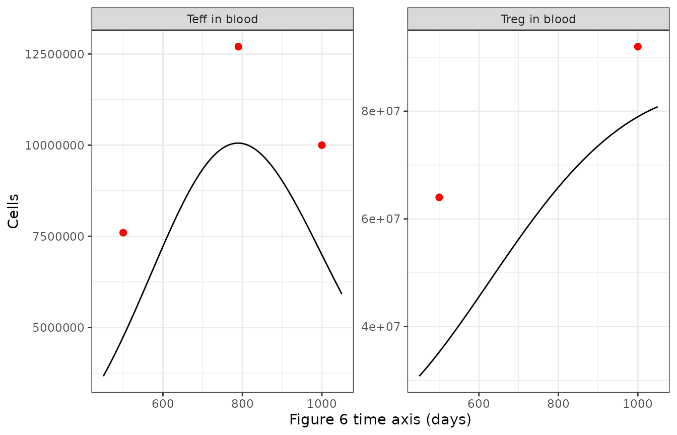
Untreated blood T cells of the packaged QSP (lines) against the digitised untreated lines of Figure 6A (points), on the Figure 6 time axis.
Both quantities have the published shape – effector T cells in blood rise to a peak and then fall as the tumour grows, regulatory T cells in blood rise steadily – and the levels agree within a factor of two, which is as close as a deterministic QSP can be expected to follow a stochastic spQSP run.
Growth-rate cases (Figures 7 and 8)
Figures 7 and 8 compare slow, medium and fast tumour growth 6 months after the pre-treatment diameter, untreated and under nivolumab. Their spatial outputs come from the ABM; the QSP solution below shows the corresponding whole-tumour behaviour for each case.
case_runs <- bind_rows(lapply(seq_len(nrow(cases)), function(i) {
  p <- c(
    k_C1_growth = cases$k_C1_growth[i], k_C_T1 = cases$k_C_T1[i], k_T1 = cases$k_T1[i],
    Treg_max = cases$Treg_max[i] * 1000 # cells/mL -> cells/L
  )
  mutate(run_case(p, days = 180), case = cases$case[i])
}))
case_sum <- case_runs |>
  filter(day >= 0) |>
  group_by(case, arm) |>
  summarise(
    t_start = t_start[1],
    diam_180 = tumour_diameter[which.min(abs(day - 180))],
    ratio_180 = (q_V_T_T1 + q_V_T_T_exh)[which.min(abs(day - 180))] / q_V_T_T0[which.min(abs(day - 180))],
    .groups = "drop"
  ) |>
  mutate(case = factor(case, levels = cases$case)) |>
  arrange(case, arm)
case_sum |>
  dplyr::rename(
    "Case" = case, "Arm" = arm, "Days to 2.255 cm" = t_start,
    "Diameter at 6 months (cm)" = diam_180, "CD8+/FoxP3+ in tumour at 6 months" = ratio_180
  ) |>
knitr::kable(digits = 2, caption = "Growth-rate cases of Table 4 (QSP layer only).")| Case | Arm | Days to 2.255 cm | Diameter at 6 months (cm) | CD8+/FoxP3+ in tumour at 6 months |
|---|---|---|---|---|
| Slow | Nivolumab 3 mg/kg q2w | 4340.21 | 0.66 | 376.33 |
| Slow | Untreated | 4340.21 | 3.03 | 2.66 |
| Medium | Nivolumab 3 mg/kg q2w | 2163.63 | 0.58 | 179.38 |
| Medium | Untreated | 2163.63 | 4.08 | 0.75 |
| Fast | Nivolumab 3 mg/kg q2w | 1440.99 | 3.23 | 3.21 |
| Fast | Untreated | 1440.99 | 5.47 | 0.44 |
cs <- split(case_sum, case_sum$arm)
stopifnot(
  # faster growth reaches the pre-treatment diameter sooner
  all(diff(cs[["Untreated"]]$t_start) < 0),
  # nivolumab raises the CD8+/FoxP3+ ratio in every case (Figure 8C)
  all(cs[["Nivolumab 3 mg/kg q2w"]]$ratio_180 > cs[["Untreated"]]$ratio_180)
)
ggplot(filter(case_runs, day >= 0), aes(day, tumour_diameter, colour = arm)) +
  geom_line(linewidth = 0.8) +
  facet_wrap(~ factor(case, levels = cases$case)) +
  labs(x = "Days from the pre-treatment diameter", y = "Tumour diameter (cm)", colour = NULL) +
  theme_bw() +
  theme(legend.position = "bottom")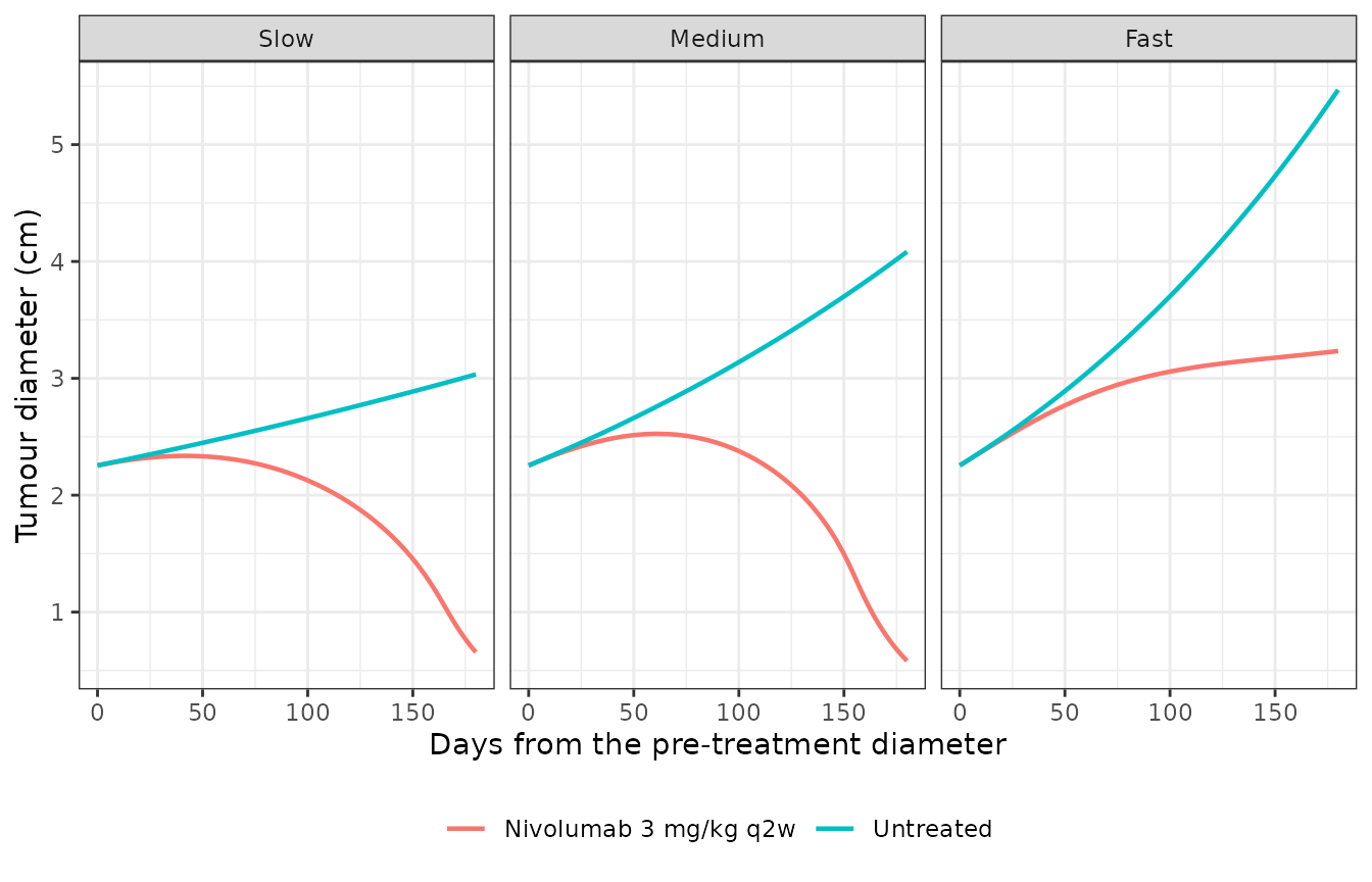
Tumour diameter after the pre-treatment diameter for the three growth-rate cases of Table 4, untreated and under nivolumab.
Nivolumab exposure
The nivolumab PK parameters are unchanged from Wang 2020 (Table S2 there, taken by those authors from Bajaj et al.). The paper reports no nivolumab exposure, so the NCA below documents the packaged model’s exposure for the first and the tenth dosing interval rather than comparing it with a published value.
nivo <- def |>
  filter(arm == "Nivolumab 3 mg/kg q2w", day >= 0, day <= 140) |>
  transmute(
    id = 1L, treatment = "Nivolumab 3 mg/kg q2w", time = day,
    conc = Cc_nivolumab * mw_nivo / 1e6 # nmol/L -> ug/mL
  ) |>
  # the growth grid and the treatment grid both end/start at day 0
  distinct(time, .keep_all = TRUE)
dose_df <- data.frame(id = 1L, treatment = "Nivolumab 3 mg/kg q2w", time = seq(0, 126, by = 14), dose = 3 * wt_kg)
o_conc <- PKNCA::PKNCAconc(nivo, conc ~ time | treatment + id)
o_dose <- PKNCA::PKNCAdose(dose_df, dose ~ time | treatment + id)
intervals <- data.frame(
  start = c(0, 126), end = c(14, 140),
  cmax = TRUE, cmin = TRUE, auclast = TRUE
)
nca <- PKNCA::pk.nca(PKNCA::PKNCAdata(o_conc, o_dose, intervals = intervals))
nca_res <- as.data.frame(nca$result)
nca_res |>
  select(start, end, PPTESTCD, PPORRES) |>
  pivot_wider(names_from = PPTESTCD, values_from = PPORRES) |>
  dplyr::rename(
    "Start (day)" = start, "End (day)" = end, "Cmax (ug/mL)" = cmax,
    "Cmin (ug/mL)" = cmin, "AUC (ug*day/mL)" = auclast
  ) |>
knitr::kable(digits = 1, caption = "Nivolumab NCA, first and tenth dosing intervals (80 kg).")| Start (day) | End (day) | AUC (ug*day/mL) | Cmax (ug/mL) | Cmin (ug/mL) |
|---|---|---|---|---|
| 0 | 14 | 307.1 | 52.7 | 13.6 |
| 126 | 140 | 685.3 | 73.9 | 36.3 |
cmin_ss <- nca_res$PPORRES[nca_res$PPTESTCD == "cmin" & nca_res$start == 126]
stopifnot(cmin_ss > 20, cmin_ss < 120)
The simulated steady-state trough of about 36 ug/mL is in the range expected for 3 mg/kg every 2 weeks (tens of ug/mL); this is a plausibility check only.
Mass conservation in the synapse
Receptor totals in the T cell : cancer cell synapse are conserved by the binding reactions (nivolumab is not consumed by binding in the SimBiology formulation), an exact identity of the ODE system.
tr <- def |> filter(arm == "Nivolumab 3 mg/kg q2w")
pd1_tot <- with(tr, q_syn_T_C1_PD1 + q_syn_T_C1_PD1_PDL1 + q_syn_T_C1_PD1_PDL2 +
  q_syn_T_C1_PD1_nivo + 2 * q_syn_T_C1_PD1_nivo_PD1)
pd1_0 <- 60000 / 151.31041193043737 * 37.8 # T_PD1_total / A_Tcell * synapse area
max(abs(pd1_tot / pd1_0 - 1))
#> [1] 6.580301e-09
stopifnot(max(abs(pd1_tot / pd1_0 - 1)) < 1e-4)
Assumptions and deviations
- Only the QSP layer is packaged. The agent-based tumour model (cancer stem-like / progenitor / senescent cells, spatial recruitment, the QSP-ABM scaling of Eqs 1-9) is stochastic and spatial and is not expressible in rxode2. The mean-field ODEs of the ABM cancer-cell lineage (S1 Supplementary Material, Eqs S2-S5) are the authors’ derivation of ABM division probabilities, not a model the paper simulates, and are not packaged either. Every figure of the paper except S1 and S2 Figs is an spQSP output, so the comparisons above are qualitative.
-
Parameter set. The S2 Table “QSP default
parameters” sheet is used; it agrees with every point value of S1 Table.
Twenty-nine of the default values are single draws inside the S1 Table
sampling ranges (for example
n_T1_clones= 61.36 in a log-normal range around 63), so the default set is one virtual patient, not a population median. The code deposit’s parameter file carries the “fast growth” case values of Table 4 (k_C1_growth0.015,k_C_T11.4,k_T10.27,Treg_max2e6 cells/mL); every other value in it agrees with the S2 Table default, six of them at higher precision than S2 Table prints (for examplek_Treg0.244055 against 0.244,k_C1_death3.00518e-5 against 3e-5, all within 0.3 percent). The printed S2 Table values are used. -
Virtual population not re-simulated. S1 and S2 Figs
show 100 virtual patients sampled from the S1 Table ranges; the ranges
are printed as “log normal [a, b]” or “log unif [a, b]” without stating
whether
ais a mean or a median or whatbscales, and the figures have no summary statistics to compare with, so the population is not regenerated here. -
Units printed in S2 Table.
q_P_durv,q_T_durv,q_LN_durvandk_cl_durvare printed in 1/second, which is inconsistent with their rate laws; the SBML-deposit units (as in Wang 2020) are used. Durvalumab is not dosed. S1 Table prints the initial lymph-node IL-2 and antigen concentrations as 1e-24 “molarity”; the SBML deposit holds 1e-24 mol per mm^3 of lymph node (1e-18 mol/L), which is what is used. -
Entinostat.
F_ENT_buccalis not in this paper and is carried from the Wang 2020 model; entinostat is not dosed here, so it affects no result. - Cancer-cell elimination event. As in Wang 2020, rxode2 has no state-reset events, so proliferation is switched off once fewer than 0.9 cancer cells remain instead of setting the count to zero.
- Dosing. Nivolumab is given as IV boluses (the infusion duration is not stated) to an 80 kg patient with a molecular weight of 144.6 kDa (S2 Table), starting at the time the tumour reaches the pre-treatment diameter.
- Figure 6 alignment. The Figure 6 time axis starts at ABM initialisation, which the paper does not relate to the QSP time origin; the digitised points were aligned at the effector T cell peak.