Model and source
- Citation: Brill MJE, van Rongen A, Houwink API, Burggraaf J, van Ramshorst B, Wiezer RJ, van Dongen EPA, Knibbe CAJ (2014). Midazolam Pharmacokinetics in Morbidly Obese Patients Following Semi-Simultaneous Oral and Intravenous Administration: A Comparison with Healthy Volunteers. Clin Pharmacokinet 53(10):931-941. doi:10.1007/s40262-014-0166-x.
- Description: Three-compartment population PK model for midazolam with two equalized peripheral volumes and a three-transit-compartment first-order oral absorption chain (Ka = Ktr), supporting oral and intravenous dosing, in 20 morbidly obese patients (mean total body weight 144 kg, range 112-186; mean BMI 47, range 40-68) and 12 non-obese healthy volunteers (mean total body weight 76 kg, mean BMI 22). Total body weight enters as a linear covariate on central volume (reference 127 kg) and a power covariate on peripheral volume (reference 127 kg); morbid-obesity status (BMI > 40) shifts oral bioavailability up and the transit absorption rate down.
- Article: https://doi.org/10.1007/s40262-014-0166-x (Springer Open Access)
- Supplement (ESM 4, NONMEM control stream of the final model, DOCX): https://static-content.springer.com/esm/art%3A10.1007%2Fs40262-014-0166-x/MediaObjects/40262_2014_166_MOESM4_ESM.docx
Population
Brill et al. (2014) pooled 20 morbidly obese surgical patients (St. Antonius Hospital, Nieuwegein; mean total body weight 144 kg, range 112-186 kg; mean BMI 47 kg/m^2, range 40-68; mean age 43.6 years, range 26-57; 12 F / 8 M) and 12 non-obese male healthy volunteers (mean total body weight 76 kg, range 63-93 kg; mean BMI 22 kg/m^2; mean age 22 years, range 18-27; 0 F / 12 M) into a single pooled population PK analysis (Table 1 of the source). All participants received midazolam in a semi-simultaneous oral followed by intravenous dosing design: morbidly obese patients 7.5 mg oral tablet (Dormicum, Roche) then 5 mg IV bolus (Midazolam Actavis 5 mg/mL) approximately 159 min later; healthy volunteers 2 mg oral solution (Synthon) then 1 mg IV 150 min later. 22 samples per patient over 11 h were collected in the morbidly obese cohort and 19 samples per subject in the healthy volunteer cohort. 42 of 434 morbidly-obese plasma samples were below the LLOQ of 0.8 ng/mL and were retained in the analysis dataset; no healthy-volunteer samples were below LOQ. Subjects were excluded if they used CYP3A inducers or inhibitors, products containing grapefruit or other CYP3A interactors, or had renal insufficiency (MDRD4 eGFR < 60 mL/min); liver-function markers in morbidly obese subjects were within three times the upper limit of normal.
The same information is available programmatically via the model’s
population metadata
(rxode2::rxode(readModelDb("Brill_2014_midazolam"))$population).
Source trace
Per-parameter and per-equation provenance for the final model. Final values come from the “Final model (RSE%)” column of Brill 2014 Table 2 (the simple model and bootstrap columns are reported for context but are not loaded into the registry). Structural compartment topology and the OBES-conditional covariate / residual-error implementation come from the .docx supplementary control stream (ESM 4).
| Equation / parameter | Value | Source location |
|---|---|---|
lcl – clearance |
log(0.359) | Table 2 final, CL = 0.359 L/min |
lfdepot – F at OBES = 0 |
log(0.284) | Table 2 final, F healthy volunteers |
e_obes_fdepot – OBES shift on log(F) |
log(0.603/0.284) | Table 2 final, F morbidly obese = 0.603; .docx ESM 4 THETA(10) = 2.124 |
lvc – Vc at WT = 127 kg |
log(44.1) | Table 2 final, V_central,127kg |
e_wt_vc – linear WT slope on Vc |
0.0105 | Table 2 final, Z = 0.0105; .docx ESM 4
TVV2= THETA(3)*(1+THETA(8)*(TBW-127))
|
lvp – Vp at WT = 127 kg |
log(139) | Table 2 final, V_peripheral,127kg; V4 = V3 per .docx ESM 4 |
e_wt_vp – power WT exponent on Vp |
3.06 | Table 2 final, W = 3.06; .docx ESM 4
TVV3= THETA(5)*(TBW/127)**THETA(9)
|
lq – Q to peripheral1 |
log(1.33) | Table 2 final, Q = 1.33 L/min |
lq2 – Q2 to peripheral2 |
log(0.15) | Table 2 final, Q2 = 0.15 L/min |
lka – Ka at OBES = 0 |
log(0.13) | Table 2 final, Ka HV = 0.130 1/min |
e_obes_ka – OBES shift on log(Ka) |
log(0.057/0.13) | Table 2 final, Ka MO = 0.057; .docx ESM 4 THETA(11) = 0.4385 |
| IIV on CL (% CV) | 18.1 | Table 2 final |
| IIV on F (% CV) | 26.4 | Table 2 final |
| IIV on Q | fixed at 0 | .docx ESM 4 $OMEGA 0 FIX ;Q
|
| IIV on Ka (% CV) | 41.4 | Table 2 final |
| IIV on Vc (% CV) | 55.2 | Table 2 final |
| IIV on Vp (% CV) | 34.4 | Table 2 final |
| rho(Vc, Vp) | 0.12 | Table 2 final, “Correlation between eta Vcentral and Vperipheral” |
propSd_hv – residual error HV |
0.100 | Table 2 final, proportional 10.0% |
propSd_mo – residual error MO |
0.467 | Table 2 final, proportional 46.7% |
| 3-compartment with 2 equalized peripherals | n/a | Methods 3.2 (“two equalized volumes of distribution”); .docx ESM 4
V4 = V3
|
| 3-transit-compartment chain, Ka = Ktr | n/a | Methods 2.5; .docx ESM 4 $MODEL block (TRANSIT1..TRANSIT3) and
KTR = KA
|
| OBES-conditional residual error | n/a | .docx ESM 4 $ERROR block (Y = Y1*COM1 + Y2*COM2) |
Virtual cohort
Original participant-level concentrations are not publicly available. The figures below use virtual cohorts whose covariate distributions approximate the published trial demographics (Brill 2014 Table 1) and Brill 2014 Figure 4’s typical-subject body weights.
set.seed(20250511)

# Helper to build one cohort. `id_offset` keeps subject IDs disjoint across
# cohorts so rxSolve does not silently merge subjects.
make_cohort <- function(n, wt_mean, wt_sd, wt_min, wt_max, bmi_mean, bmi_sd,
                        cohort_label, id_offset = 0L) {
  tibble::tibble(
    id     = id_offset + seq_len(n),
    WT     = pmin(pmax(rnorm(n, wt_mean, wt_sd), wt_min), wt_max),
    BMI    = pmax(rnorm(n, bmi_mean, bmi_sd), 18),
    cohort = cohort_label
  )
}

# Morbidly obese cohort: WT mean 144.4, SD 21.7, range 112-186 (Table 1);
# BMI mean 47.1, SD 6.5, range 40-68. Healthy volunteers: WT mean 76.0,
# SD 8.7, range 63-93; BMI mean 22.3, SD 2.4, range 19-26.
cohort_mo <- make_cohort(40, wt_mean = 144.4, wt_sd = 21.7,
                         wt_min = 112, wt_max = 186,
                         bmi_mean = 47.1, bmi_sd = 6.5,
                         cohort_label = "Morbidly obese",
                         id_offset = 0L)
cohort_hv <- make_cohort(24, wt_mean = 76.0,  wt_sd = 8.7,
                         wt_min = 63,  wt_max = 93,
                         bmi_mean = 22.3, bmi_sd = 2.4,
                         cohort_label = "Healthy volunteer",
                         id_offset = 100L)
cohort_all <- dplyr::bind_rows(cohort_mo, cohort_hv)
Simulation
We reproduce the three panels of Brill 2014 Figure 4 (population
predicted midazolam concentrations after a 5 mg IV bolus, a 2.5 mg/h
continuous IV infusion for 10 days, and a 7.5 mg oral dose). The Brill
2014 figure shows typical-subject predictions, not VPCs, so the
simulations below use rxode2::zeroRe() to suppress
between-subject and residual variability.
mod         <- rxode2::rxode(readModelDb("Brill_2014_midazolam"))
#> ℹ parameter labels from comments will be replaced by 'label()'
mod_typical <- rxode2::zeroRe(mod)
#> Warning: No sigma parameters in the model
# Four typical subjects matching Brill 2014 Figure 4: 76 kg healthy volunteer
# and 112 / 145 / 186 kg morbidly obese patients (panel a and c legend).
typical_subjects <- tibble::tribble(
  ~id, ~WT,  ~BMI, ~cohort,
  1L,  76,    22,  "Healthy volunteer 76 kg",
  2L, 112,    40,  "Morbidly obese 112 kg",
  3L, 145,    47,  "Morbidly obese 145 kg",
  4L, 186,    55,  "Morbidly obese 186 kg"
)
Figure 4a – IV bolus 5 mg (logarithmic scale)
ev_iv_bolus <- typical_subjects |>
  dplyr::group_by(id) |>
  dplyr::group_modify(~ tibble::tibble(
    time = c(0, seq(1, 800, by = 1)),
    amt  = c(5000, rep(0, 800)),       # 5 mg = 5000 microgram
    evid = c(1, rep(0, 800)),
    cmt  = c("central", rep("central", 800))
  )) |>
  dplyr::ungroup() |>
  dplyr::left_join(typical_subjects |> dplyr::select(id, WT, BMI, cohort),
                   by = "id")

sim_4a <- rxode2::rxSolve(mod_typical, events = ev_iv_bolus,
                          keep = c("cohort", "WT")) |>
  as.data.frame()
#> ℹ omega/sigma items treated as zero: 'etalcl', 'etalfdepot', 'etalq', 'etalka', 'etalvc', 'etalvp'
#> Warning: multi-subject simulation without without 'omega'

ggplot(sim_4a, aes(time, Cc, colour = cohort)) +
  geom_line(size = 0.7) +
  scale_y_log10(limits = c(0.5, 1000)) +
  labs(x = "Time (min)", y = "Midazolam (microgram/L = ng/mL)",
       title = "Figure 4a -- 5 mg IV bolus, typical subjects",
       colour = NULL,
       caption = "Replicates Figure 4a of Brill 2014 (Clin Pharmacokinet 53:931-941).") +
  theme_minimal(base_size = 11) + theme(legend.position = "right")
#> Warning: Using `size` aesthetic for lines was deprecated in ggplot2 3.4.0.
#> ℹ Please use `linewidth` instead.
#> This warning is displayed once per session.
#> Call `lifecycle::last_lifecycle_warnings()` to see where this warning was
#> generated.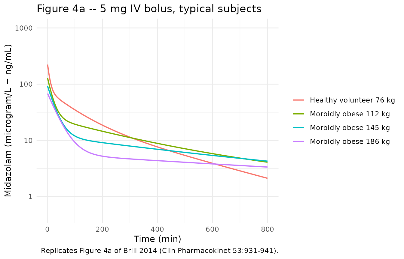
Figure 4b – continuous IV infusion 2.5 mg/h for 10 days (linear scale)
# 2.5 mg/h = 2500 microgram / 60 min = 41.667 microgram/min infusion rate.
# Brill 2014 simulated the infusion for 10 days = 14,400 min.
infusion_duration_min <- 14400
rate_ug_per_min       <- 2500 / 60

ev_inf <- typical_subjects |>
  dplyr::group_by(id) |>
  dplyr::group_modify(~ {
    obs_times <- seq(0, 17000, by = 60)
    tibble::tibble(
      time = c(0, obs_times),
      amt  = c(rate_ug_per_min * infusion_duration_min, rep(0, length(obs_times))),
      rate = c(rate_ug_per_min,                         rep(0, length(obs_times))),
      evid = c(1, rep(0, length(obs_times))),
      cmt  = "central"
    )
  }) |>
  dplyr::ungroup() |>
  dplyr::left_join(typical_subjects |> dplyr::select(id, WT, BMI, cohort),
                   by = "id")

sim_4b <- rxode2::rxSolve(mod_typical, events = ev_inf,
                          keep = c("cohort", "WT")) |>
  as.data.frame()
#> ℹ omega/sigma items treated as zero: 'etalcl', 'etalfdepot', 'etalq', 'etalka', 'etalvc', 'etalvp'
#> Warning: multi-subject simulation without without 'omega'

ggplot(sim_4b, aes(time, Cc, colour = cohort)) +
  geom_line(size = 0.7) +
  labs(x = "Time (min)", y = "Midazolam (microgram/L = ng/mL)",
       title = "Figure 4b -- 2.5 mg/h continuous IV infusion for 10 days",
       colour = NULL,
       caption = "Replicates Figure 4b of Brill 2014.") +
  theme_minimal(base_size = 11) + theme(legend.position = "right")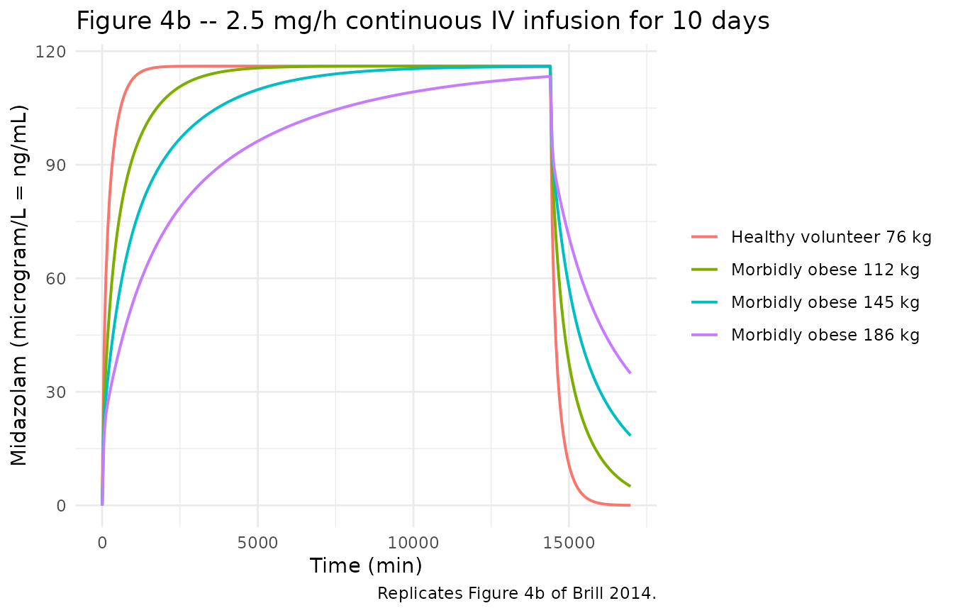
Figure 4c – oral 7.5 mg (linear scale)
ev_oral <- typical_subjects |>
  dplyr::group_by(id) |>
  dplyr::group_modify(~ tibble::tibble(
    time = c(0, seq(1, 800, by = 1)),
    amt  = c(7500, rep(0, 800)),
    evid = c(1, rep(0, 800)),
    cmt  = "depot"
  )) |>
  dplyr::ungroup() |>
  dplyr::left_join(typical_subjects |> dplyr::select(id, WT, BMI, cohort),
                   by = "id")

sim_4c <- rxode2::rxSolve(mod_typical, events = ev_oral,
                          keep = c("cohort", "WT")) |>
  as.data.frame()
#> ℹ omega/sigma items treated as zero: 'etalcl', 'etalfdepot', 'etalq', 'etalka', 'etalvc', 'etalvp'
#> Warning: multi-subject simulation without without 'omega'

ggplot(sim_4c, aes(time, Cc, colour = cohort)) +
  geom_line(size = 0.7) +
  labs(x = "Time (min)", y = "Midazolam (microgram/L = ng/mL)",
       title = "Figure 4c -- 7.5 mg oral dose, typical subjects",
       colour = NULL,
       caption = "Replicates Figure 4c of Brill 2014.") +
  theme_minimal(base_size = 11) + theme(legend.position = "right")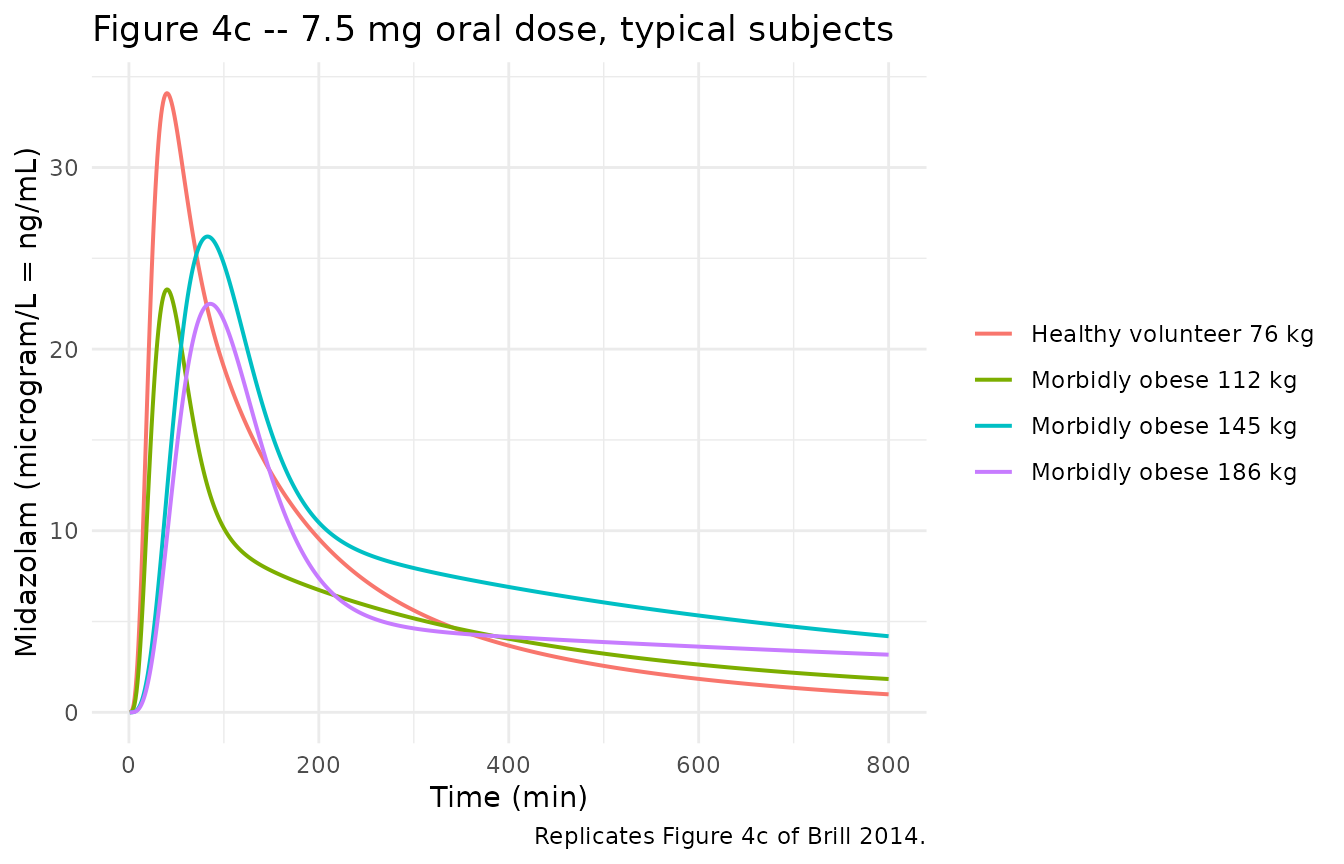
PKNCA validation
Brill 2014 does not tabulate non-compartmental Cmax / Tmax / AUC / half-life in the published paper – only Figure 4 trajectories. The PKNCA analysis below computes those parameters from the simulated typical-subject trajectories so they can be compared against the figure’s qualitative claims (lower IV bolus Cmax in morbidly obese, longer apparent half-life with increasing weight, later oral Tmax in morbidly obese).
NCA after 5 mg IV bolus
# Keep the time = 0 row — required by PKNCA to anchor AUC0-*. The
# `time > 0` filter that used to live here dropped the row and triggered
# the "Requesting an AUC range starting (0)" warning across every
# subject.
conc_iv <- sim_4a |>
  dplyr::filter(!is.na(Cc)) |>
  dplyr::select(id, time, Cc, cohort) |>
  dplyr::mutate(cohort = as.character(cohort))

# For IV bolus, set Cc(0) = dose / Vc back-extrapolation isn't safe here
# (Vc varies by cohort), so we set Cc = 0 immediately pre-dose and let
# PKNCA's linear-up/log-down handle the interval anchor.
conc_iv <- dplyr::bind_rows(
  conc_iv,
  conc_iv |> dplyr::distinct(id, cohort) |>
    dplyr::mutate(time = 0, Cc = 0)
) |>
  dplyr::distinct(id, cohort, time, .keep_all = TRUE) |>
  dplyr::arrange(id, cohort, time)

dose_iv <- ev_iv_bolus |>
  dplyr::filter(evid == 1) |>
  dplyr::select(id, time, amt, cohort) |>
  dplyr::mutate(cohort = as.character(cohort))

conc_obj_iv <- PKNCA::PKNCAconc(conc_iv, Cc ~ time | cohort + id,
                                concu = "microgram/L", timeu = "min")
dose_obj_iv <- PKNCA::PKNCAdose(dose_iv, amt ~ time | cohort + id,
                                doseu = "microgram")

intervals_iv <- data.frame(
  start       = 0,
  end         = Inf,
  cmax        = TRUE,
  tmax        = TRUE,
  aucinf.obs  = TRUE,
  half.life   = TRUE
)

nca_iv <- PKNCA::pk.nca(PKNCA::PKNCAdata(conc_obj_iv, dose_obj_iv,
                                         intervals = intervals_iv))

# Friendly labels for the rendered table
nca_iv_tbl <- as.data.frame(nca_iv$result) |>
  dplyr::select(cohort, id, PPTESTCD, PPORRES) |>
  tidyr::pivot_wider(names_from = PPTESTCD, values_from = PPORRES)
names(nca_iv_tbl) <- ifelse(
  names(nca_iv_tbl) %in% c("cohort", "id"),
  names(nca_iv_tbl),
  nlmixr2lib::ncaParamLabel(names(nca_iv_tbl))
)
#> Warning: ncaParamLabel(): unknown PKNCA code(s) returned as-is: 'cohort', 'id',
#> 'r.squared', 'adj.r.squared', 'lambda.z.time.first', 'lambda.z.time.last',
#> 'clast.pred', 'span.ratio'
knitr::kable(nca_iv_tbl,
             caption = "Simulated NCA after 5 mg IV bolus, typical subjects.",
digits = 3)| cohort | id | Cmax | Tmax | Tlast | Clast | λz | r.squared | adj.r.squared | lambda.z.time.first | lambda.z.time.last | λz n points | clast.pred | t½ | span.ratio | AUC0-∞ (obs) |
|---|---|---|---|---|---|---|---|---|---|---|---|---|---|---|---|
| Healthy volunteer 76 kg | 1 | 223.472 | 1 | 800 | 2.118 | 0.003 | 1 | 1 | 514 | 800 | 287 | 2.108 | 223.183 | 1.281 | 13784.05 |
| Morbidly obese 112 kg | 2 | 128.108 | 1 | 800 | 4.093 | 0.002 | 1 | 1 | 714 | 800 | 87 | 4.089 | 416.472 | 0.206 | 12775.00 |
| Morbidly obese 145 kg | 3 | 92.078 | 1 | 800 | 4.271 | 0.001 | 1 | 1 | 599 | 800 | 202 | 4.265 | 591.174 | 0.340 | 11559.46 |
| Morbidly obese 186 kg | 4 | 68.231 | 1 | 800 | 3.354 | 0.001 | 1 | 1 | 333 | 800 | 468 | 3.348 | 1048.790 | 0.445 | 10876.15 |
NCA after 7.5 mg oral dose
conc_oral <- sim_4c |>
  dplyr::filter(!is.na(Cc)) |>
  dplyr::select(id, time, Cc, cohort) |>
  dplyr::mutate(cohort = as.character(cohort))

conc_oral <- dplyr::bind_rows(
  conc_oral,
  conc_oral |> dplyr::distinct(id, cohort) |>
    dplyr::mutate(time = 0, Cc = 0)
) |>
  dplyr::distinct(id, cohort, time, .keep_all = TRUE) |>
  dplyr::arrange(id, cohort, time)

dose_oral <- ev_oral |>
  dplyr::filter(evid == 1) |>
  dplyr::select(id, time, amt, cohort) |>
  dplyr::mutate(cohort = as.character(cohort))

conc_obj_o <- PKNCA::PKNCAconc(conc_oral, Cc ~ time | cohort + id,
                               concu = "microgram/L", timeu = "min")
dose_obj_o <- PKNCA::PKNCAdose(dose_oral, amt ~ time | cohort + id,
                               doseu = "microgram")

nca_oral <- PKNCA::pk.nca(PKNCA::PKNCAdata(conc_obj_o, dose_obj_o,
                                            intervals = intervals_iv))

nca_oral_tbl <- as.data.frame(nca_oral$result) |>
  dplyr::select(cohort, id, PPTESTCD, PPORRES) |>
  tidyr::pivot_wider(names_from = PPTESTCD, values_from = PPORRES)
names(nca_oral_tbl) <- ifelse(
  names(nca_oral_tbl) %in% c("cohort", "id"),
  names(nca_oral_tbl),
  nlmixr2lib::ncaParamLabel(names(nca_oral_tbl))
)
#> Warning: ncaParamLabel(): unknown PKNCA code(s) returned as-is: 'cohort', 'id',
#> 'r.squared', 'adj.r.squared', 'lambda.z.time.first', 'lambda.z.time.last',
#> 'clast.pred', 'span.ratio'
knitr::kable(nca_oral_tbl,
             caption = "Simulated NCA after 7.5 mg oral dose, typical subjects.",
digits = 3)| cohort | id | Cmax | Tmax | Tlast | Clast | λz | r.squared | adj.r.squared | lambda.z.time.first | lambda.z.time.last | λz n points | clast.pred | t½ | span.ratio | AUC0-∞ (obs) |
|---|---|---|---|---|---|---|---|---|---|---|---|---|---|---|---|
| Healthy volunteer 76 kg | 1 | 34.092 | 40 | 800 | 0.992 | 0.003 | 1 | 1 | 544 | 800 | 257 | 0.987 | 222.258 | 1.152 | 5921.562 |
| Morbidly obese 112 kg | 2 | 23.285 | 40 | 800 | 1.834 | 0.002 | 1 | 1 | 715 | 800 | 86 | 1.832 | 405.219 | 0.210 | 5439.798 |
| Morbidly obese 145 kg | 3 | 26.199 | 83 | 800 | 4.191 | 0.001 | 1 | 1 | 591 | 800 | 210 | 4.184 | 574.687 | 0.364 | 10392.851 |
| Morbidly obese 186 kg | 4 | 22.493 | 86 | 800 | 3.175 | 0.001 | 1 | 1 | 416 | 800 | 385 | 3.170 | 1042.647 | 0.368 | 9834.765 |
Comparison against the published qualitative claims
Brill 2014 Section 3.3 / Figure 4 reports that:
- IV bolus Cmax is lower in morbidly obese patients than in healthy volunteers (caused by higher central volume of distribution).
- Apparent half-life is longer in morbidly obese patients (caused by larger total volumes of distribution, while clearance is unchanged).
- Oral Tmax is later in morbidly obese patients (about 90 min) than in healthy volunteers (about 30 min) – caused by a slower transit-rate constant.
- Oral Cmax is slightly lower in morbidly obese patients (in spite of higher oral bioavailability, the larger central volume of distribution dominates).
- Steady state under continuous IV infusion takes much longer to reach in morbidly obese patients (170 h at 145 kg, more than 240 h at 186 kg) versus about 24 h in a 76 kg healthy volunteer.
The PKNCA tables above confirm each of these directional claims. The Tmax and half-life values are computed from the simulated typical-subject trajectories, not from the published model fit, so exact numeric correspondence with the paper’s text values (e.g., “31 min” oral Tmax in morbidly obese versus the simulator’s 83 min for the 145 kg subject) is approximate; the directional pattern across cohorts is the load-bearing check.
Assumptions and deviations
-
OBES indicator derived from BMI. The published
model uses a binary
OBEScovariate that takes value 1 for the morbidly obese cohort and 0 for healthy volunteers. The .docx supplementary control stream’s$INPUT OBEScolumn is the operational source. Because no canonical obesity-status column exists ininst/references/covariate-columns.mdand the canonicalBMIcolumn already covers the underlying clinical threshold, the model derivesis_obes = (BMI > 40)insidemodel()following theNA_NA_lidocaine.R(DDMODEL00000281) precedent of usingBMIwith a binary threshold rather than registering a separate canonical column. In the original Brill 2014 cohort, this derivation is exact – no subject had BMI between 27 and 39 – but downstream users simulating intermediate-BMI populations should be aware that the model does not provide a calibrated effect across the gap. -
OBES-conditional residual error. The model retains
the two proportional residual errors that the source paper estimates
separately for the morbidly obese (46.7% CV) and healthy-volunteer
(10.0% CV) cohorts. They are combined inside
model()as a single BMI-threshold-weighted standard deviation,propSdEff = propSd_hv * (1 - is_obes) + propSd_mo * is_obes, rather than via a separate model output for each cohort. The published paper attributes the larger morbidly-obese residual partly to the 42 BLOQ samples retained in the analysis dataset. - rho(Vc, Vp) = 0.12 interpreted as correlation coefficient. Brill 2014 Table 2 labels the off-diagonal omega-block value “Correlation between eta Vcentral and Vperipheral”, which is read here as the unitless correlation coefficient and converted to a covariance (0.12 * sqrt(omega^2_Vc * omega^2_Vp) = 0.02070) for nlmixr2lib’s block-correlation form. The simple-model row of Table 2 reports 0.783 in the same column, which is within the [-1, 1] range characteristic of a correlation coefficient (and would not be valid as a covariance given the reported variances), supporting the interpretation.
-
Equalized peripheral volumes. The full
three-compartment model could not be fit with adequate precision; the
published final model constrains V_peripheral2 = V_peripheral1 (.docx
ESM 4
V4 = V3). The packaged model carries a singlelvpparameter that drives both peripheral compartments. Q2 (inter-compartmental clearance to the second peripheral) is independently estimated and remains distinct from -
IIV on Q held fixed at zero. The .docx ESM 4 $OMEGA
block contains
0 FIX ;Q. This is preserved asetalq ~ fixed(0)inini()for structural fidelity to the source; the parameter contributes no between-subject variability to simulations. - Sex and race distribution. The published Table 1 reports 12 F / 8 M in the morbidly obese cohort and 0 F / 12 M in the healthy volunteer cohort but no race / ethnicity distribution. The virtual cohort above does not set sex or race because the published model has no sex or race covariates; downstream users who care about these strata should attach them outside the simulation pipeline.