Model and source
#> ℹ parameter labels from comments will be replaced by 'label()'- Citation: Li TF, Hu L, Ma XL, Huang L, Liu XM, Luo XX, Feng WY, Wu CF. Population pharmacokinetics of cyclosporine in Chinese children receiving hematopoietic stem cell transplantation. Acta Pharmacol Sin. 2019;40(12):1603-1610. doi:10.1038/s41401-019-0277-x
- Description: One-compartment intravenous population PK model for cyclosporine A in Chinese children receiving allogeneic haematopoietic stem cell transplantation (Li 2019), with allometric body-weight scaling on CL and V, linear post-operative-day effects on CL and V, a power eGFR effect and a fractional triazole-antifungal effect on CL, CYP3A4*1G (rs2242480) genotype multipliers on CL, and combined proportional plus additive residual error.
- Article: https://doi.org/10.1038/s41401-019-0277-x
Li and colleagues fitted a one-compartment model with first-order elimination to 1010 whole-blood cyclosporine A (CsA) trough concentrations from 86 Chinese children who received intravenous CsA (2 h infusion every 12 h) around allogeneic haematopoietic stem cell transplantation (allo-HSCT). Clearance carries allometric weight scaling, a linear post-operative-day (POD) effect, a power effect of eGFR, a fractional reduction with concomitant triazole antifungals (TAF), and CYP3A4*1G (rs2242480) genotype multipliers; volume carries allometric weight scaling and a linear POD effect.
mod <- readModelDb("Li_2019_cyclosporine")
mod
#> function() {
#>   description <- "One-compartment intravenous population PK model for cyclosporine A in Chinese children receiving allogeneic haematopoietic stem cell transplantation (Li 2019), with allometric body-weight scaling on CL and V, linear post-operative-day effects on CL and V, a power eGFR effect and a fractional triazole-antifungal effect on CL, CYP3A4*1G (rs2242480) genotype multipliers on CL, and combined proportional plus additive residual error."
#>   reference <- "Li TF, Hu L, Ma XL, Huang L, Liu XM, Luo XX, Feng WY, Wu CF. Population pharmacokinetics of cyclosporine in Chinese children receiving hematopoietic stem cell transplantation. Acta Pharmacol Sin. 2019;40(12):1603-1610. doi:10.1038/s41401-019-0277-x"
#>   vignette <- "Li_2019_cyclosporine"
#>   units <- list(time = "h", dosing = "mg", concentration = "ng/mL")
#>
#>   compartmentData <- list(
#>     # Li 2019 Abstract: "Whole blood samples were collected" and the CMIA
#>     # (Architect i2000SR) cyclosporine assay is a whole-blood assay, so the
#>     # modelled matrix is whole blood.
#>     central = list(analyte = "cyclosporine", units = "mg", specimen = "whole blood", verified = TRUE)
#>   )
#>
#>   covariateData <- list(
#>     WT = list(
#>       description = "Body weight",
#>       units = "kg",
#>       type = "continuous",
#>       reference_category = NULL,
#>       notes = paste(
#>         "Allometric scaling (WT / 70)^0.75 on CL and (WT / 70)^1 on V, both",
#>         "exponents fixed (Li 2019 Eq. 3 and text: 'PWR is the allometric",
#>         "coefficient fixed at a value of 0.75 for clearance and a value of 1",
#>         "for distribution volume'). Cohort mean 31.93 kg, median 28.8 kg",
#>         "(Table 1). The Results text gives the range 6.5-69.0 kg while",
#>         "Table 1 gives 9.4-78.5 kg; the source does not resolve the",
#>         "discrepancy."
#>       ),
#>       source_name = "WT"
#>     ),
#>     POD = list(
#>       description = "Post-operative day (days since allogeneic HSCT)",
#>       units = "days",
#>       type = "continuous",
#>       reference_category = NULL,
#>       notes = paste(
#>         "Time-varying. Enters CL and V as the linear deviation",
#>         "(1 - (POD - 9) * theta) (Li 2019 Eq. 4 and Eq. 5), so both",
#>         "parameters decline linearly with POD; the centring value 9 days is",
#>         "printed in the equations. Table 1: mean 29.7, median 25, range",
#>         "0-67 days. Cyclosporine was started on Day -7 or -10; how the",
#>         "pre-transplant troughs were coded is not stated, but Table 1's",
#>         "lower bound of 0 suggests they carried POD = 0. The V factor reaches",
#>         "zero at POD = 9 + 1 / 0.0197 = 59.8 days and is negative beyond, so",
#>         "the published equation is only usable for POD below about 50 days",
#>         "(the model does not truncate it)."
#>       ),
#>       source_name = "POD"
#>     ),
#>     CRCL = list(
#>       description = "Estimated glomerular filtration rate, BSA-normalised",
#>       units = "mL/min/1.73 m^2",
#>       type = "continuous",
#>       reference_category = NULL,
#>       notes = paste(
#>         "Power effect (eGFR / 172.46)^0.545 on CL (Li 2019 Eq. 4); 172.46 is",
#>         "the Table 1 cohort median (mean 179.4, range 24.93-377.54). The",
#>         "estimating equation for eGFR is not stated in the paper (a",
#>         "creatinine-based paediatric equation such as bedside Schwartz is",
#>         "the usual choice; Table 1 reports serum creatinine in umol/L)."
#>       ),
#>       source_name = "eGFR"
#>     ),
#>     CONMED_AZOLE = list(
#>       description = "Concomitant triazole antifungal (1 = yes, 0 = no)",
#>       units = "(binary)",
#>       type = "binary",
#>       reference_category = "0 (no triazole antifungal)",
#>       notes = paste(
#>         "Li 2019 'TAF' indicator ('patients were coadministered of TAF, the",
#>         "TAF = 1, otherwise TAF = 0'); fractional effect (1 - 0.36 * TAF) on",
#>         "CL (Eq. 4). The pooled triazoles were voriconazole (61 children),",
#>         "itraconazole (19), posaconazole (6) and fluconazole (1); only 4",
#>         "children never received one (Table 1). The paper does not say",
#>         "whether TAF was coded per record (time-varying) or per subject."
#>       ),
#>       source_name = "TAF"
#>     ),
#>     SNP_CYP3A4_RS2242480_VAR_COUNT = list(
#>       description = "CYP3A4*1G (rs2242480) variant (T) allele count: 0 = CC, 1 = CT, 2 = TT",
#>       units = "(count, 0/1/2 alleles per subject)",
#>       type = "continuous",
#>       reference_category = NULL,
#>       notes = paste(
#>         "Li 2019 codes the genotype as 'Gene' = 1 for CC, 2 for TT and 3 for",
#>         "CT (Table 3 footnote) and multiplies CL by 0.984 for Gene = 1 and by",
#>         "1.22 for Gene = 2 or 3 (Results text below Eq. 5; Table 3 rows",
#>         "'Gene-1/2/3 ON CL'). Canonical mapping: CC -> 0, CT -> 1, TT -> 2.",
#>         "Table 2: CC 50 (61.0%), CT 26 (31.7%), TT 6 (7.3%); the T allele is",
#>         "the minor allele (frequency 23.2%). 82 of 86 children were",
#>         "genotyped; how the 4 ungenotyped children were coded is not",
#>         "reported, so no missing-genotype indicator is carried."
#>       ),
#>       source_name = "Gene"
#>     )
#>   )
#>
#>   covariatesDataExcluded <- list(
#>     AGE = list(
#>       description = "Age",
#>       units = "years",
#>       type = "continuous",
#>       notes = "Table 1 mean 8.38 (1.1-16.8). Screened; the age trend in CL disappeared after allometric weight scaling (Fig. 1)."
#>     ),
#>     SEXF = list(
#>       description = "Female sex indicator",
#>       units = "(binary)",
#>       type = "binary",
#>       reference_category = "0 (male)",
#>       notes = "30 of 86 female (Table 1). Screened, not retained."
#>     ),
#>     HGB = list(
#>       description = "Haemoglobin",
#>       units = "g/L",
#>       type = "continuous",
#>       notes = "Table 1 mean 85.49 g/L. Screened, not retained."
#>     ),
#>     HCT = list(
#>       description = "Haematocrit",
#>       units = "%",
#>       type = "continuous",
#>       notes = "Table 1 mean 24.42%. Screened, not retained."
#>     ),
#>     ALB = list(
#>       description = "Serum albumin",
#>       units = "g/L",
#>       type = "continuous",
#>       notes = "Table 1 mean 34.98 (printed with the unit 'U/L'). Screened, not retained."
#>     ),
#>     SNP_CYP3A5_RS776746 = list(
#>       description = "CYP3A5*3 (rs776746) genotype",
#>       units = "(genotype)",
#>       type = "categorical",
#>       notes = "Table 2: CC 42 / CT 34 / TT 5. Screened, not significant (Discussion)."
#>     )
#>   )
#>
#>   population <- list(
#>     species = "human",
#>     n_subjects = 86L,
#>     n_studies = 1L,
#>     n_observations = 1010L,
#>     age_range = "1.1-16.8 years",
#>     age_mean = "8.38 years (SD 3.78; median 8.35)",
#>     weight_range = "9.4-78.5 kg (Table 1; the Results text gives 6.5-69.0 kg)",
#>     weight_median = "28.8 kg (mean 31.93, SD 16.75)",
#>     sex_female_pct = 34.9,
#>     race_ethnicity = "Chinese (single centre, Beijing)",
#>     disease_state = "Children with malignant haematological disorders (ALL 33.7%, AA 26.7%, AML 25.6%, NHL 5.8%, MDS 4.7%, other 3.5%) receiving allogeneic haematopoietic stem cell transplantation",
#>     dose_range = "Intravenous cyclosporine as a 2 h infusion every 12 h from Day -7 or -10, initial 2-3 mg/kg, then adjusted to a trough target of 150-250 ng/mL; per-dose amount mean 28.6 mg (median 25, range 5-125 mg)",
#>     regions = "China (Peking University People's Hospital, Beijing)",
#>     cyp3a4_1g_distribution = "rs2242480 CC 50 (61.0%), CT 26 (31.7%), TT 6 (7.3%) of 82 genotyped",
#>     pod_range = "0-67 days (mean 29.7, median 25)",
#>     egfr_median = "172.46 mL/min/1.73 m^2 (range 24.93-377.54)",
#>     notes = "Retrospective therapeutic-drug-monitoring data: 1010 whole-blood troughs (mean 12 per child) drawn before the morning intravenous infusion and measured by chemiluminescent microparticle immunoassay (LLOQ 30 ng/mL). Fit by NONMEM VII FOCE-I."
#>   )
#>
#>   ini({
#>     # Structural parameters at the Eq. 4 / Eq. 5 reference subject: 70 kg,
#>     # POD 9 days, eGFR 172.46 mL/min/1.73 m^2, no triazole antifungal. The
#>     # CYP3A4*1G multiplier (0.984 CC / 1.22 T carrier) is applied on top of
#>     # the printed CL for every genotype, so no genotype reproduces CL = 42.3
#>     # exactly. Li 2019 Table 3 'Final model Estimate (RSE%)'.
#>     #
#>     # The data are trough-only, so V is identified from accumulation across
#>     # days; the resulting typical half-life is long (about 50 h at 70 kg),
#>     # as in the sibling Feng 2023 cyclosporine model.
#>     lcl <- log(42.3); label("Typical clearance CL at 70 kg, POD 9 d, eGFR 172.46, no triazole (L/h)") # Li 2019 Table 3: CL = 42.3 L/h (RSE 10.6%)
#>     lvc <- log(3100); label("Typical volume of distribution V at 70 kg, POD 9 d (L)") # Li 2019 Table 3: V = 3100 L (RSE 13.1%)
#>
#>     # Allometric exponents fixed (Li 2019 Eq. 3 and text).
#>     e_wt_cl <- fixed(0.75); label("Allometric exponent of (WT / 70) on CL (unitless)") # Li 2019 Methods 'Covariate analysis': PWR fixed at 0.75 for clearance
#>     e_wt_vc <- fixed(1); label("Allometric exponent of (WT / 70) on V (unitless)") # Li 2019 Methods 'Covariate analysis': PWR fixed at 1 for distribution volume
#>
#>     # Covariate effects, Li 2019 Eq. 4 and Eq. 5:
#>     #   CL = CLpop * (WT/70)^0.75 * (1 - theta_TAF * TAF) * (1 - (POD - 9) * theta_POD_CL)
#>     #        * (eGFR / 172.46)^theta_eGFR * exp(eta), then * 0.984 (CC) or * 1.22 (CT, TT)
#>     #   V  = Vpop * (WT/70) * (1 - (POD - 9) * theta_POD_V) * exp(eta)
#>     e_azole_cl <- 0.36; label("Fractional decrease in CL with a concomitant triazole antifungal (unitless)") # Li 2019 Table 3: theta TAF-CL = 0.36 (RSE 16.3%)
#>     e_pod_cl <- 0.00703; label("Fractional decrease in CL per post-operative day above 9 d (1/day)") # Li 2019 Table 3: theta POD-CL = 0.00703 (RSE 21.5%)
#>     e_pod_vc <- 0.0197; label("Fractional decrease in V per post-operative day above 9 d (1/day)") # Li 2019 Table 3: theta POD-V = 0.0197 (RSE 29.8%)
#>     e_crcl_cl <- 0.545; label("Power exponent of (eGFR / 172.46) on CL (unitless)") # Li 2019 Table 3: theta eGFR-CL = 0.545 (RSE 29.9%)
#>     e_cyp3a4_wild_cl <- 0.984; label("CL multiplier for CYP3A4*1G (rs2242480) CC (unitless)") # Li 2019 Table 3: Gene-1 ON CL = 0.984 (RSE 8.1%); Gene 1 = CC
#>     e_cyp3a4_varhom_cl <- 1.22; label("CL multiplier for CYP3A4*1G (rs2242480) TT (unitless)") # Li 2019 Table 3: Gene-2 ON CL = 1.22 (RSE 10.1%); Gene 2 = TT
#>     e_cyp3a4_het_cl <- 1.22; label("CL multiplier for CYP3A4*1G (rs2242480) CT (unitless)") # Li 2019 Table 3: Gene-3 ON CL = 1.22 (RSE 8.9%); Gene 3 = CT
#>
#>     # Inter-individual variability, exponential (Li 2019 Eq. 1). Table 3
#>     # labels the rows 'omega^2', so they are variances:
#>     #   CL 0.0744 -> CV 27.8%;  V 0.454 -> CV 73.6%
#>     etalcl ~ 0.0744 # Li 2019 Table 3: omega^2 CL = 0.0744 (RSE 19.5%, shrinkage 8.4%)
#>     etalvc ~ 0.454 # Li 2019 Table 3: omega^2 V = 0.454 (RSE 24%, shrinkage 27.2%)
#>
#>     # Residual error, Li 2019 Eq. 2: Cobs = Cpred * (1 + eps1) + eps2. Table 3
#>     # heads the rows 'sigma^2 1 (%)' = 0.154 and 'sigma^2 2 (ng/mL)' = 30.3.
#>     # The units printed (ng/mL, not (ng/mL)^2) and the Results text ('the
#>     # additive error was 30.3 ng/mL') identify these as standard deviations;
#>     # the text's 'proportional error was 22.9%' is the RSE column of the same
#>     # row. See the vignette for the scale decision and the Figure 2b check.
#>     propSd <- 0.154; label("Proportional residual error (fraction)") # Li 2019 Table 3: sigma 1 = 0.154 (RSE 22.9%); read as an SD
#>     addSd <- 30.3; label("Additive residual error (ng/mL)") # Li 2019 Table 3: sigma 2 = 30.3 ng/mL (RSE 21.7%); Results text 'additive error was 30.3 ng/mL'
#>   })
#>   model({
#>     # 1. CYP3A4*1G genotype multiplier (Li 2019 Results text below Eq. 5):
#>     # CC -> 0.984, CT or TT -> 1.22.
#>     cyp3a4_cl <- e_cyp3a4_wild_cl * (SNP_CYP3A4_RS2242480_VAR_COUNT == 0) +
#>       e_cyp3a4_het_cl * (SNP_CYP3A4_RS2242480_VAR_COUNT == 1) +
#>       e_cyp3a4_varhom_cl * (SNP_CYP3A4_RS2242480_VAR_COUNT == 2)
#>
#>     # 2. Individual parameters (Li 2019 Eq. 4 and Eq. 5)
#>     cl <- exp(lcl + etalcl) * (WT / 70)^e_wt_cl * (1 - e_azole_cl * CONMED_AZOLE) *
#>       (1 - (POD - 9) * e_pod_cl) * (CRCL / 172.46)^e_crcl_cl * cyp3a4_cl
#>     vc <- exp(lvc + etalvc) * (WT / 70)^e_wt_vc * (1 - (POD - 9) * e_pod_vc)
#>
#>     # 3. Micro-constant and ODE. All modelled troughs followed intravenous
#>     # 2 h infusions (Li 2019 'CsA administration'), so doses enter central.
#>     kel <- cl / vc
#>     d/dt(central) <- -kel * central
#>
#>     # 4. Observation: mg / L * 1000 = ng/mL
#>     Cc <- 1000 * central / vc
#>     Cc ~ add(addSd) + prop(propSd)
#>   })
#> }
#> <environment: 0x55aa128f43d8>
Population
| Field | Value |
|---|---|
| species | human |
| n_subjects | 86 |
| n_studies | 1 |
| n_observations | 1010 |
| age_range | 1.1-16.8 years |
| age_mean | 8.38 years (SD 3.78; median 8.35) |
| weight_range | 9.4-78.5 kg (Table 1; the Results text gives 6.5-69.0 kg) |
| weight_median | 28.8 kg (mean 31.93, SD 16.75) |
| sex_female_pct | 34.9 |
| race_ethnicity | Chinese (single centre, Beijing) |
| disease_state | Children with malignant haematological disorders (ALL 33.7%, AA 26.7%, AML 25.6%, NHL 5.8%, MDS 4.7%, other 3.5%) receiving allogeneic haematopoietic stem cell transplantation |
| dose_range | Intravenous cyclosporine as a 2 h infusion every 12 h from Day -7 or -10, initial 2-3 mg/kg, then adjusted to a trough target of 150-250 ng/mL; per-dose amount mean 28.6 mg (median 25, range 5-125 mg) |
| regions | China (Peking University People’s Hospital, Beijing) |
| cyp3a4_1g_distribution | rs2242480 CC 50 (61.0%), CT 26 (31.7%), TT 6 (7.3%) of 82 genotyped |
| pod_range | 0-67 days (mean 29.7, median 25) |
| egfr_median | 172.46 mL/min/1.73 m^2 (range 24.93-377.54) |
| notes | Retrospective therapeutic-drug-monitoring data: 1010 whole-blood troughs (mean 12 per child) drawn before the morning intravenous infusion and measured by chemiluminescent microparticle immunoassay (LLOQ 30 ng/mL). Fit by NONMEM VII FOCE-I. |
The cohort was 86 children (56 boys, 30 girls) aged 1.1-16.8 years (mean 8.38) at Peking University People’s Hospital, transplanted for acute lymphocytic leukaemia (33.7 %), aplastic anaemia (26.7 %), acute myeloid leukaemia (25.6 %) and other haematological disorders. Median body weight was 28.8 kg and median eGFR 172.46 mL/min/1.73 m^2. Almost every child received a triazole antifungal at some point (voriconazole 61, itraconazole 19, posaconazole 6, fluconazole 1; none in 4). CYP3A4*1G genotypes among the 82 genotyped children were CC 50, CT 26 and TT 6 (Li 2019 Tables 1-2).
Source trace
| Equation / parameter | Value | Source location |
|---|---|---|
lcl |
42.3 L/h | Table 3 ‘CL (L/h)’ (RSE 10.6 %) |
lvc |
3100 L | Table 3 ‘V (L)’ (RSE 13.1 %) |
e_wt_cl |
0.75 (fixed) | Methods ‘Covariate analysis’, Eq. 3 |
e_wt_vc |
1 (fixed) | Methods ‘Covariate analysis’, Eq. 3 |
e_azole_cl |
0.36 | Table 3 ‘theta TAF-CL’ (RSE 16.3 %); Eq. 4 |
e_pod_cl |
0.00703 /day | Table 3 ‘theta POD-CL’ (RSE 21.5 %); Eq. 4 |
e_pod_vc |
0.0197 /day | Table 3 ‘theta POD-V’ (RSE 29.8 %); Eq. 5 |
e_crcl_cl |
0.545 | Table 3 ‘theta eGFR-CL’ (RSE 29.9 %); Eq. 4 |
e_cyp3a4_wild_cl |
0.984 | Table 3 ‘Gene-1 ON CL’ (RSE 8.1 %); Gene 1 = CC (Table 3 footnote) |
e_cyp3a4_varhom_cl |
1.22 | Table 3 ‘Gene-2 ON CL’ (RSE 10.1 %); Gene 2 = TT |
e_cyp3a4_het_cl |
1.22 | Table 3 ‘Gene-3 ON CL’ (RSE 8.9 %); Gene 3 = CT |
etalcl |
0.0744 | Table 3 ‘omega^2 CL’ (shrinkage 8.4 %) |
etalvc |
0.454 | Table 3 ‘omega^2 V’ (shrinkage 27.2 %) |
propSd |
0.154 | Table 3 ‘sigma^2 1 (%)’ (see Assumptions) |
addSd |
30.3 ng/mL | Table 3 ‘sigma^2 2 (ng/mL)’; Results ‘the additive error was 30.3 ng/mL’ |
cl <- ... |
n/a | Eq. 4 and the genotype sentence below Eq. 5 |
vc <- ... |
n/a | Eq. 5 |
| Exponential IIV | n/a | Eq. 1 |
Cc ~ add(addSd) + prop(propSd) |
n/a | Eq. 2, Cobs = Cpred * (1 + eps1) + eps2
|
One compartment, IV dosing into central
|
n/a | Results; Methods ‘CsA administration’ |
Cc <- 1000 * central / vc |
n/a | Unit conversion mg/L to ng/mL |
Equations 4 and 5 are typeset as display maths; they read
CL_i = CL_pop * (WT_i/70)^0.75 * (1 - theta_TAF-CL * TAF)
       * (1 - (POD - 9) * theta_POD-CL) * (eGFR/172.46)^theta_eGFR-CL * exp(eta_i)
V_i  = V_pop * (WT_i/70) * (1 - (POD - 9) * theta_POD-V) * exp(eta_i)
followed by “If the gene is 1, CL_i = CL_i*0.984; If the gene is 2 or 3, CL_i = CL_i*1.22”.
Structural checks
These checks use typical values only (zeroRe()), so they
are deterministic.
mod_typ <- rxode2::zeroRe(mod)
#> ℹ parameter labels from comments will be replaced by 'label()'

probe_params <- function(WT, POD, CRCL, AZOLE, GENO) {
  d <- data.frame(
    id = 1L, time = c(0, 1), evid = c(1L, 0L), amt = c(1, NA_real_),
    cmt = "central", WT = WT, POD = POD, CRCL = CRCL,
    CONMED_AZOLE = AZOLE, SNP_CYP3A4_RS2242480_VAR_COUNT = GENO
  )
  out <- as.data.frame(rxode2::rxSolve(mod_typ, d))
  c(cl = out$cl[1], vc = out$vc[1])
}

# 1. At the Eq. 4/5 reference (70 kg, POD 9, eGFR 172.46, no TAF) the model
#    returns the printed CL times the genotype multiplier, and the printed V.
ref_cc <- probe_params(70, 9, 172.46, 0, 0)
#> ℹ omega/sigma items treated as zero: 'etalcl', 'etalvc'
ref_ct <- probe_params(70, 9, 172.46, 0, 1)
#> ℹ omega/sigma items treated as zero: 'etalcl', 'etalvc'
ref_tt <- probe_params(70, 9, 172.46, 0, 2)
#> ℹ omega/sigma items treated as zero: 'etalcl', 'etalvc'
stopifnot(
  abs(ref_cc[["cl"]] - 42.3 * 0.984) < 1e-8,
  abs(ref_ct[["cl"]] - 42.3 * 1.22) < 1e-8,
  abs(ref_tt[["cl"]] - 42.3 * 1.22) < 1e-8,
  abs(ref_cc[["vc"]] - 3100) < 1e-8
)

# 2. Discussion: CL in T-allele carriers 'increased by 24.5% compared with
#    that in CYP3A4*1G CC carriers'. The rounded Table 3 multipliers give
#    1.22 / 0.984 = 1.240.
t_vs_cc <- ref_ct[["cl"]] / ref_cc[["cl"]]
stopifnot(abs(t_vs_cc - 1.245) < 0.01)

# 3. Results: 'The weight-normalized clearance was 0.75 L/h/kg'. Evaluated at
#    the Table 1 median weight (28.8 kg) and the Eq. 4 reference covariates.
med_cc <- probe_params(28.8, 9, 172.46, 0, 0)
#> ℹ omega/sigma items treated as zero: 'etalcl', 'etalvc'
cl_per_kg <- c(
  `no genotype factor` = 42.3 * (28.8 / 70)^0.75 / 28.8,
  `CC (model)` = med_cc[["cl"]] / 28.8
)
stopifnot(all(abs(cl_per_kg / 0.75 - 1) < 0.02))
round(c(t_vs_cc = t_vs_cc, cl_per_kg), 4)
#>            t_vs_cc no genotype factor         CC (model)
#>             1.2398             0.7545             0.7424
The printed weight-normalised clearance (0.75 L/h/kg) is reproduced at the median body weight, which confirms that the allometric reference is 70 kg with the 0.75 exponent and that CL is in L/h (not L/h per kg).
pod_grid <- data.frame(POD = c(0, 9, 25, 40, 55))
pod_grid$cl_factor <- 1 - (pod_grid$POD - 9) * 0.00703
pod_grid$v_factor <- 1 - (pod_grid$POD - 9) * 0.0197
pod_grid$cl_model <- vapply(pod_grid$POD, function(p) probe_params(70, p, 172.46, 0, 0)[["cl"]], 0) / (42.3 * 0.984)
#> ℹ omega/sigma items treated as zero: 'etalcl', 'etalvc'
#> ℹ omega/sigma items treated as zero: 'etalcl', 'etalvc'
#> ℹ omega/sigma items treated as zero: 'etalcl', 'etalvc'
#> ℹ omega/sigma items treated as zero: 'etalcl', 'etalvc'
#> ℹ omega/sigma items treated as zero: 'etalcl', 'etalvc'
pod_grid$v_model <- vapply(pod_grid$POD, function(p) probe_params(70, p, 172.46, 0, 0)[["vc"]], 0) / 3100
#> ℹ omega/sigma items treated as zero: 'etalcl', 'etalvc'
#> ℹ omega/sigma items treated as zero: 'etalcl', 'etalvc'
#> ℹ omega/sigma items treated as zero: 'etalcl', 'etalvc'
#> ℹ omega/sigma items treated as zero: 'etalcl', 'etalvc'
#> ℹ omega/sigma items treated as zero: 'etalcl', 'etalvc'
stopifnot(
  all(abs(pod_grid$cl_model - pod_grid$cl_factor) < 1e-10),
  all(abs(pod_grid$v_model - pod_grid$v_factor) < 1e-10)
)
pod_grid |>
  dplyr::select(POD, cl_model, v_model) |>
  dplyr::rename(
    "POD (days)" = POD,
    "CL / CL(POD 9)" = cl_model,
    "V / V(POD 9)" = v_model
  ) |>
knitr::kable(digits = 3, caption = "Post-operative-day factors on CL and V (Li 2019 Eq. 4 and Eq. 5).")| POD (days) | CL / CL(POD 9) | V / V(POD 9) |
|---|---|---|
| 0 | 1.063 | 1.177 |
| 9 | 1.000 | 1.000 |
| 25 | 0.888 | 0.685 |
| 40 | 0.782 | 0.389 |
| 55 | 0.677 | 0.094 |
Both factors decline linearly with POD. The V factor falls to 0.19 by POD 50 and would reach zero at POD 59.8, so the published equation should not be used beyond about POD 50 (see Assumptions).
Virtual cohort
The cohort reproduces the Table 1 and Table 2 marginals. Body weight is drawn log-normally around the 28.8 kg median and redrawn (not clamped) outside the Table 1 range; eGFR is drawn log-normally around its 172.46 median. The paper reports no joint distribution, so covariates are drawn independently.
set.seed(2019)
n_sub <- 200L

draw_in_range <- function(n, med, sdlog, lo, hi) {
  x <- med * exp(stats::rnorm(n, 0, sdlog))
  bad <- x < lo | x > hi
  while (any(bad)) {
    x[bad] <- med * exp(stats::rnorm(sum(bad), 0, sdlog))
    bad <- x < lo | x > hi
  }
  x
}

subj <- tibble::tibble(
  id = seq_len(n_sub),
  WT = draw_in_range(n_sub, 28.8, 0.5, 9.4, 78.5),
  CRCL = draw_in_range(n_sub, 172.46, 0.2, 24.93, 377.54),
  # 82 of 86 children received a triazole antifungal (Table 1)
  CONMED_AZOLE = stats::rbinom(n_sub, 1, 82 / 86),
  # Table 2 genotype frequencies: CC 50, CT 26, TT 6 of 82
  SNP_CYP3A4_RS2242480_VAR_COUNT = sample(0:2, n_sub, replace = TRUE, prob = c(50, 26, 6) / 82)
)
summary(subj[, -1])
#>        WT              CRCL        CONMED_AZOLE
#>  Min.   : 9.938   Min.   :103.2   Min.   :0.000
#>  1st Qu.:19.834   1st Qu.:148.3   1st Qu.:1.000
#>  Median :26.124   Median :167.3   Median :1.000
#>  Mean   :29.711   Mean   :172.6   Mean   :0.955
#>  3rd Qu.:37.802   3rd Qu.:196.7   3rd Qu.:1.000
#>  Max.   :78.233   Max.   :273.3   Max.   :1.000
#>  SNP_CYP3A4_RS2242480_VAR_COUNT
#>  Min.   :0.00
#>  1st Qu.:0.00
#>  Median :0.00
#>  Mean   :0.46
#>  3rd Qu.:1.00
#>  Max.   :2.00
Simulation
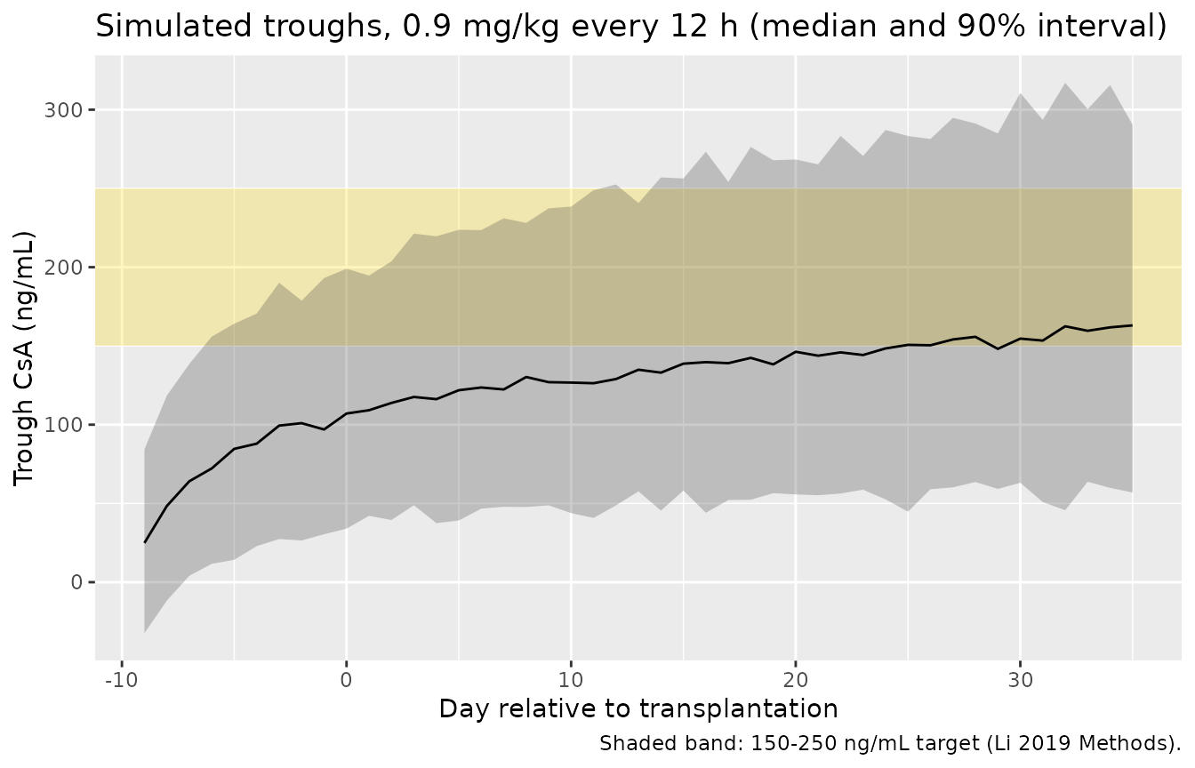
Dosing follows the Methods: a 2 h intravenous infusion every 12 h, started nine days before transplantation (the paper gives Day -7 or -10). The per-dose amount is 0.9 mg/kg, i.e. the Table 1 mean dose (28.6 mg) divided by the mean body weight (31.93 kg); in the study the dose was titrated to troughs of 150-250 ng/mL, which a fixed-dose simulation does not reproduce subject by subject. POD is time-varying: pre-transplant records carry POD = 0.
start_day <- -9
n_days <- 45
dose_times <- seq(0, 24 * n_days - 12, by = 12)
trough_times <- dose_times[-1] - 0.01 # immediately before each morning/evening dose
obs_grid <- sort(unique(c(0, trough_times, seq(0, 24 * n_days, by = 2))))

pod_at <- function(time) pmax(0, floor(time / 24) + start_day)

dose_rows <- tidyr::expand_grid(subj, time = dose_times) |>
  dplyr::mutate(evid = 1L, amt = 0.9 * WT, rate = amt / 2, cmt = "central")
obs_rows <- tidyr::expand_grid(subj, time = obs_grid) |>
  dplyr::mutate(evid = 0L, amt = NA_real_, rate = NA_real_, cmt = "central")
events <- dplyr::bind_rows(dose_rows, obs_rows) |>
  dplyr::mutate(POD = pod_at(time)) |>
  dplyr::arrange(id, time, dplyr::desc(evid)) |>
  as.data.frame()
rxode2::rxSetSeed(20190277)
sim <- rxode2::rxSolve(
  mod, events,
  keep = c("WT", "CRCL", "CONMED_AZOLE", "SNP_CYP3A4_RS2242480_VAR_COUNT", "POD")
) |>
  as.data.frame()
#> ℹ parameter labels from comments will be replaced by 'label()'

troughs <- sim |>
  dplyr::filter(round(time %% 12, 2) == 11.99) |>
  dplyr::mutate(day_post_tx = floor(time / 24) + start_day)
Trough concentrations over time (cf. Figures 2 and 3)
Figure 2 of Li 2019 shows observed troughs mostly between about 50 and 400 ng/mL (bulk 100-300 ng/mL) over 0-1800 h from the first dose.
troughs |>
  dplyr::group_by(day_post_tx) |>
  dplyr::summarise(
    p05 = quantile(sim, 0.05), p50 = median(sim), p95 = quantile(sim, 0.95),
    .groups = "drop"
  ) |>
  ggplot(aes(day_post_tx, p50)) +
  annotate("rect", xmin = -Inf, xmax = Inf, ymin = 150, ymax = 250, fill = "gold", alpha = 0.25) +
  geom_ribbon(aes(ymin = p05, ymax = p95), alpha = 0.25) +
  geom_line() +
  labs(
    x = "Day relative to transplantation", y = "Trough CsA (ng/mL)",
    title = "Simulated troughs, 0.9 mg/kg every 12 h (median and 90% interval)",
    caption = "Shaded band: 150-250 ng/mL target (Li 2019 Methods)."
  )
# Trough over the bulk of the observation window (POD 10-40; Table 1 median
# POD 25). A mis-transcribed CL, V or unit moves the median by a factor of
# several; the window is the observed bulk in Figure 2, not a tuned target.
window <- troughs |> dplyr::filter(day_post_tx >= 10, day_post_tx <= 40)
trough_median <- median(window$sim)
trough_median_ipred <- median(window$Cc)
c(median_DV = trough_median, median_IPRED = trough_median_ipred)
#>    median_DV median_IPRED
#>     145.2673     144.7756
stopifnot(trough_median > 100, trough_median < 300)
With the cohort-mean dose the typical trough lands inside the 150-250 ng/mL target the clinicians titrated to, consistent with the Figure 2 scatter.
PKNCA: steady-state dosing interval
The paper reports no NCA; PKNCA is used here to characterise a steady-state interval (day 20 post-transplant, POD 20) by CYP3A4*1G group, and to confirm that the long half-life makes the trough close to the interval average.
tau_start <- 24 * (20 - start_day)
conc_nca <- sim |>
  dplyr::filter(time >= tau_start, time <= tau_start + 12, !is.na(Cc)) |>
  dplyr::mutate(
    time = time - tau_start,
    treatment = ifelse(SNP_CYP3A4_RS2242480_VAR_COUNT == 0, "CYP3A4*1G CC", "CYP3A4*1G T carrier")
  ) |>
  dplyr::select(id, time, Cc, treatment)
# Guarantee an exact time-zero row per subject (pre-dose trough)
stopifnot(all(tapply(conc_nca$time, conc_nca$id, min) == 0))

dose_nca <- conc_nca |>
  dplyr::distinct(id, treatment) |>
  dplyr::left_join(dplyr::select(subj, id, WT), by = "id") |>
  dplyr::mutate(time = 0, amt = 0.9 * WT)

conc_obj <- PKNCA::PKNCAconc(conc_nca, Cc ~ time | treatment + id, concu = "ng/mL", timeu = "h")
dose_obj <- PKNCA::PKNCAdose(dose_nca, amt ~ time | treatment + id, doseu = "mg")
intervals <- data.frame(start = 0, end = 12, cmax = TRUE, cmin = TRUE, auclast = TRUE, cav = TRUE)
nca_res <- PKNCA::pk.nca(PKNCA::PKNCAdata(conc_obj, dose_obj, intervals = intervals))
nca_tab <- as.data.frame(nca_res) |>
  dplyr::group_by(treatment, PPTESTCD) |>
  dplyr::summarise(median = median(PPORRES), .groups = "drop") |>
  tidyr::pivot_wider(names_from = PPTESTCD, values_from = median)
nca_tab |>
  dplyr::rename(
    "Group" = treatment,
    "AUC0-12 (ng*h/mL)" = auclast,
    "Cavg (ng/mL)" = cav,
    "Cmax (ng/mL)" = cmax,
    "Cmin (ng/mL)" = cmin
  ) |>
knitr::kable(digits = 1, caption = "Median steady-state NCA on POD 20 (simulated, 0.9 mg/kg every 12 h).")| Group | AUC0-12 (ng*h/mL) | Cavg (ng/mL) | Cmax (ng/mL) | Cmin (ng/mL) |
|---|---|---|---|---|
| CYP3A4*1G CC | 2030.5 | 169.2 | 184.2 | 153.5 |
| CYP3A4*1G T carrier | 1693.6 | 141.1 | 161.9 | 127.7 |
# The T-carrier group has the 1.24-fold higher CL, so a lower exposure. The
# genotype is the only systematic difference between groups; the median
# ratio is a centre statistic (not an extreme), with wide headroom.
ratio <- nca_tab$auclast[nca_tab$treatment == "CYP3A4*1G CC"] /
  nca_tab$auclast[nca_tab$treatment == "CYP3A4*1G T carrier"]
stopifnot(ratio > 1)
ratio
#> [1] 1.19897
Residual error scale
Table 3 heads the residual rows sigma^2 1 (%) = 0.154
and sigma^2 2 (ng/mL) = 30.3, while the Results text says
“the proportional error was 22.9 %, and the additive error was 30.3
ng/mL”. 22.9 % is the RSE printed next to 0.154, so the text quotes the
RSE column for the proportional term; its additive figure, and the ng/mL
unit (not (ng/mL)^2), treat the Table 3 estimates as standard
deviations. The two readings imply very different residual spreads:
ipred <- c(50, 200, 350)
ruv <- tibble::tibble(
  `IPRED (ng/mL)` = ipred,
  `SD, as SDs (0.154, 30.3)` = sqrt((0.154 * ipred)^2 + 30.3^2),
  `SD, as variances (0.392, 5.5)` = sqrt((sqrt(0.154) * ipred)^2 + 30.3)
)
knitr::kable(ruv, digits = 1)| IPRED (ng/mL) | SD, as SDs (0.154, 30.3) | SD, as variances (0.392, 5.5) |
|---|---|---|
| 50 | 31.3 | 20.4 |
| 200 | 43.2 | 78.7 |
| 350 | 61.8 | 137.5 |
In Figure 2b (DV vs IPRED) the bulk of the observations at IPRED =
200 ng/mL lie within roughly 120-290 ng/mL, a residual SD of about 40-50
ng/mL, which agrees with the standard-deviation reading (43 ng/mL) and
not the variance reading (78 ng/mL). The model therefore uses
propSd = 0.154 and addSd = 30.3 ng/mL.
Assumptions and deviations
-
Residual error scale. Table 3 labels the residual
rows
sigma^2; they are encoded as standard deviations for the reasons given above. - POD centring and range. Eq. 4 and 5 centre POD at 9 days and apply a linear decline. The V factor becomes zero at POD 59.8 and negative beyond, inside the observed POD range (0-67); the model reproduces the equation as printed and does not truncate it, so it should not be simulated past about POD 50. The Discussion describes CL rising over the first 9 days and then falling, but the printed linear form is monotonically decreasing; the equation is implemented as printed.
- Pre-transplant records. CsA started on Day -7 or -10 while Table 1 reports POD 0-67; the simulations here code pre-transplant days as POD = 0.
- Genotype coding. Gene 1 = CC, 2 = TT, 3 = CT (Table 3 footnote) is mapped to the canonical variant-allele count (CC 0, CT 1, TT 2). The printed CL is multiplied by 0.984 or 1.22 for every genotype, so no genotype has exactly CL = 42.3 L/h. Handling of the 4 ungenotyped children is not reported, and no missing-genotype term is included.
- eGFR equation. Not stated in the paper; the model expects the same BSA-normalised units (mL/min/1.73 m^2) with the cohort median 172.46.
- Triazole indicator. Voriconazole, itraconazole, posaconazole and fluconazole are pooled into one indicator with one effect, as in the paper.
- Body weight range. The Results text gives 6.5-69.0 kg and Table 1 gives 9.4-78.5 kg; the virtual cohort uses the Table 1 range.
- Dosing in the simulations. A fixed 0.9 mg/kg per dose (Table 1 mean dose over mean weight) replaces the paper’s trough-guided titration, so the simulated trough distribution is wider than the titrated clinical data.
- Covariate independence. The paper reports only marginals; covariates are drawn independently.