Rupatadine (Santamaria 2017)
Source:vignettes/articles/Santamaria_2017_rupatadine.Rmd
Santamaria_2017_rupatadine.RmdModel and source
#> ℹ parameter labels from comments will be replaced by 'label()'Citation: Santamaria E, Estevez JA, Riba J, Izquierdo I, Valle M. Population pharmacokinetic modelling of rupatadine solution in 6-11 year olds and optimisation of the experimental design in younger children. PLoS ONE. 2017;12(4):e0176091. doi:10.1371/journal.pone.0176091
Description: Two-compartment population PK model with first-order absorption and an absorption lag time for oral rupatadine 1 mg/mL solution in 6-11 year old children with allergic rhinitis, with a linear-additive body-weight effect on apparent clearance (Santamaria 2017)
Santamaria and colleagues fitted a population PK model to rupatadine
oral solution in 6-11 year old children with allergic rhinitis, and then
used that model for two downstream purposes: selecting a dose for a
planned study in 2-5 year olds, and optimising the blood-sampling design
of that study. Only the population PK model is packaged here. The
design-optimisation exercise (the paper’s Tables 1 and 4, produced in
WinPOPT) is a study-design calculation rather than a model and has no
representation in nlmixr2lib.
Population
The model was built from an open-label, single-dose study in eleven children aged 6-11 years with a history of allergic rhinitis, conducted in Australia (Royal Children’s Hospital, Melbourne; Peninsula Private Hospital and Peninsula Clinical Research Centre, Rivercity). Eligibility required a body weight of at least 16 kg, and children taking medication that could significantly interact with CYP3A4 were excluded, since rupatadine is mainly metabolised by that enzyme.
Baseline demographics (Santamaria 2017 Table 2): 5 male / 6 female; age 7.94-11.93 years (median 10.41); body weight 22.0-68.5 kg (median 38.5); height 1.18-1.59 m (median 1.44); BMI 13.4-27.1 kg/m^2 (median 18.54). Each child gave a full concentration-time profile, with 8 samples at predose and 0.5, 1, 2, 4, 8, 12 and 24 h after a single oral dose of rupatadine 1 mg/mL solution: 2.5 mg (2.5 mL) for children weighing more than 10 and less than 25 kg, and 5 mg (5 mL) for children weighing 25 kg or more. All but two children weighed more than 25 kg and therefore received 5 mg. A total of 84 plasma concentrations entered the analysis; concentrations below the limit of quantification in the elimination phase (12% of observations) were discarded. The observed rupatadine concentration range was 0.1-4.9 ng/mL.
The same information is available programmatically via
rxode2::rxode(readModelDb("Santamaria_2017_rupatadine"))$population.
| Field | Value |
|---|---|
| species | human |
| n_subjects | 11 |
| n_studies | 1 |
| n_observations | 84 |
| age_range | 7.94-11.93 years |
| age_median | 10.41 years |
| weight_range | 22.0-68.5 kg |
| weight_median | 38.5 kg |
| height_range | 1.18-1.59 m |
| height_median | 1.44 m |
| bmi_range | 13.4-27.1 kg/m^2 |
| bmi_median | 18.54 kg/m^2 |
| sex_female_pct | 54.5 |
| race_ethnicity | Not reported in source |
| disease_state | Allergic rhinitis, otherwise in good health |
| dose_range | Single oral dose of rupatadine 1 mg/mL solution; 2.5 mg (2.5 mL) for children weighing more than 10 and less than 25 kg, 5 mg (5 mL) for children weighing 25 kg or more. Nine of the eleven children received 5 mg. |
| regions | Australia (Royal Children’s Hospital, Melbourne; Peninsula Private Hospital and Peninsula Clinical Research Centre, Rivercity) |
| co_medication | Participants who had taken any medication that could significantly interact with CYP3A4 were excluded, as rupatadine is mainly metabolised by that enzyme. |
| notes | Open-label single-dose study in children 6-11 years of age weighing at least 16 kg with a history of allergic rhinitis (Santamaria 2017 Material and methods, ‘Population’; demographics in Table 2). A full concentration-time profile was obtained for each child, with 8 samples per child at predose and 0.5, 1, 2, 4, 8, 12 and 24 h postdose. 84 plasma concentrations entered the analysis; concentrations below the limit of quantification in the elimination phase (12 percent of observations) were discarded. Observed rupatadine concentration range 0.1-4.9 ng/mL. Bioanalysis by validated LC-MS/MS with clomipramine as internal standard; within- and between-run precision error below 12.71 percent and accuracy-related errors within plus or minus 12.83 percent. Estimation by FOCE in NONMEM. The same final model was then used to select a 2.5 mg dose and to optimise the sampling design for a planned study in 2-5 year olds; that design optimisation (WinPOPT, paper Tables 1 and 4) is a study-design exercise rather than a model and is not represented here. |
Source trace
Per-parameter provenance is recorded as an in-file comment beside
each ini() entry in
inst/modeldb/specificDrugs/Santamaria_2017_rupatadine.R.
The table collects them in one place. Every value is from the
Final Model column of Santamaria 2017 Table 3; the
parenthesised figure in that table is the relative standard error in
percent, which the model file records in the comment but does not
encode.
| Equation / parameter | Value | Source location |
|---|---|---|
lka (ka) |
0.53 1/h | Table 3, final model, ka (h-1) (RSE 15) |
ltlag (tlag) |
0.22 h | Table 3, final model, Lag time (h) (RSE 13) |
lcl (theta1) |
225 L/h | Table 3, final model, CL/F (L/h), theta1 (RSE 63) |
e_wt_cl (theta2) |
333 L/h | Table 3, final model, CL/F (L/h), theta2 (RSE 44) |
lvc (Vc/F) |
108 L | Table 3, final model, Vc/F (L) (RSE 52) |
lq (CLd/F) |
209 L/h | Table 3, final model, CLd/F (L/h) (RSE 30) |
lvp (Vp/F) |
1430 L | Table 3, final model, Vp/F (L) (RSE 56) |
etalcl |
0.16 (= 0.40^2) | Table 3, final model, IIV CL/F (%) = 40 (RSE 25) |
etalvc |
0.8798 (= 0.938^2) | Table 3, final model, IIV Vc/F (%) = 93.8 (RSE 38) |
addSd |
0.18 ng/mL | Table 3, final model, Residual error (ng/mL) (RSE
41) |
Clearance covariate model
CL = theta1 + theta2 * WEIGHT/38.5
|
n/a | Table 3 footnote, and the display equation in Results, “Covariate inclusion” |
IIV model CL_i = CL_pop * exp(eta_i), eta mean 0
variance omega^2 |
n/a | Material and methods, “Population analysis”, display equation |
| Two-compartment disposition, first-order absorption, absorption lag | n/a | Results, “Population analysis”; Conclusions |
| Additive residual error | n/a | Results, “Population analysis” |
| Reference weight 38.5 kg | n/a | Table 2 median body weight, used as the normalising constant in the Table 3 footnote equation |
Two features of this model are worth flagging because they differ from the common popPK pattern.
The body-weight effect on clearance is linear-additive, not
allometric. The authors state explicitly that “although an
allometric scaling model was tested, the function that best described
the weight-CL/F relationship was a linear model”, and print
CL = theta1 + theta2 * WEIGHT/38.5. Both thetas carry units
of L/h. The model file therefore puts the weight-independent intercept
in the canonical lcl and the weight slope in
e_wt_cl (which here is an L/h slope, not the dimensionless
exponent that name carries in allometric models), and adds them on the
linear scale inside model(). This is the encoding
prescribed by inst/references/parameter-names.md for a
covariate expression with a positive intercept; the precedent in the
registry is Blair_2004_raltitrexed.
Every disposition parameter is apparent. Rupatadine
undergoes extensive CYP3A4 first-pass metabolism, so CL/F,
Vc/F, CLd/F and Vp/F all absorb
an unknown, small bioavailability. That is why the typical clearance
(558 L/h) and peripheral volume (1430 L) look large for a child.
Bioavailability is not separately identifiable from oral-only data and
is not a parameter of the model.
Structural checks against published values
These two checks are deterministic: they use the typical-value model
(rxode2::zeroRe()), so both sides of each comparison come
from the same solved trajectory and a tight bound is the correct
one.
mod <- readModelDb("Santamaria_2017_rupatadine")

# Weights spanning the simulated 2-5 year old range plus the 6-11 year old
# cohort median, which is the reference weight of the clearance model.
wt_grid <- c(10, 15, 20, 24, 38.5)

ev_typ <- dplyr::bind_rows(lapply(seq_along(wt_grid), function(i) {
  e <- rxode2::et(amt = 5, cmt = "depot")
  e <- rxode2::et(e, seq(0, 96, by = 0.05))
  e <- as.data.frame(e)
  e$id <- i
  e$WT <- wt_grid[i]
  e
}))

sim_typ <- rxode2::rxSolve(rxode2::zeroRe(mod), ev_typ, keep = "WT") |>
  as.data.frame()
#> ℹ parameter labels from comments will be replaced by 'label()'
#> ℹ omega/sigma items treated as zero: 'etalcl', 'etalvc'
#> Warning: multi-subject simulation without without 'omega'
Check 1 – typical clearance reproduces the paper’s printed regression
The paper’s Discussion states that “according to our final model, the estimated value of CL/F for a typical 6-11 year old weighting 38.5 kg would be 558 l/h”. The check below compares the clearance the solver actually computed against the paper’s printed equation at every weight, so it goes red if the intercept, the slope, the normalising weight, or the additive-versus-multiplicative form were mis-transcribed.
cl_chk <- sim_typ |>
  dplyr::group_by(WT) |>
  dplyr::summarise(cl_model = mean(cl), .groups = "drop") |>
  # Santamaria 2017 Table 3 footnote: CL = theta1 + theta2 * WEIGHT/38.5.
  dplyr::mutate(
    cl_paper = 225 + 333 * WT / 38.5,
    pct_diff = 100 * (cl_model - cl_paper) / cl_paper
  )

cl_chk |>
  dplyr::rename(
    "Body weight (kg)" = WT,
    "CL/F from model (L/h)" = cl_model,
    "CL/F from printed equation (L/h)" = cl_paper,
    "% difference" = pct_diff
  ) |>
knitr::kable(digits = 4, caption = "Typical apparent clearance versus the paper's printed weight regression.")| Body weight (kg) | CL/F from model (L/h) | CL/F from printed equation (L/h) | % difference |
|---|---|---|---|
| 10.0 | 311.4935 | 311.4935 | 0 |
| 15.0 | 354.7403 | 354.7403 | 0 |
| 20.0 | 397.9870 | 397.9870 | 0 |
| 24.0 | 432.5844 | 432.5844 | 0 |
| 38.5 | 558.0000 | 558.0000 | 0 |
# Deterministic: both sides are the same algebraic form, so the only difference
# is floating-point. Realised 0 at 2 / 4 / 16 solver threads.
stopifnot(max(abs(cl_chk$pct_diff)) < 1e-6)

# The paper's own stated value for a typical 38.5 kg child.
cl_385 <- cl_chk$cl_model[cl_chk$WT == 38.5]
stopifnot(abs(cl_385 - 558) < 0.5)
The typical clearance at the cohort median weight is 558.0 L/h, matching the 558 L/h the paper reports.
Check 2 – AUC x CL mass balance
For a linear model with complete absorption into the system,
AUC(0-inf) * CL/F = Dose, exactly and at any weight.
Comparing the PKNCA integral against the solver’s own clearance
therefore validates the ODE encoding and the mg-to-ng/mL unit
scaling in one number. A discrepancy of more than a fraction of a
percent means the concentration scaling, the dose units, or the
compartment structure is wrong.
nca_typ <- sim_typ |>
  dplyr::filter(!is.na(Cc)) |>
  dplyr::select(id, time, Cc, WT)

# Guarantee a time-zero record per subject; pre-dose concentration after an
# extravascular dose is zero.
nca_typ <- dplyr::bind_rows(
  nca_typ,
  nca_typ |> dplyr::distinct(id, WT) |> dplyr::mutate(time = 0, Cc = 0)
) |>
  dplyr::distinct(id, time, .keep_all = TRUE) |>
  dplyr::arrange(id, time)

dose_typ <- sim_typ |>
  dplyr::distinct(id, WT) |>
  dplyr::mutate(time = 0, amt = 5)

nca_typ_res <- PKNCA::pk.nca(PKNCA::PKNCAdata(
  PKNCA::PKNCAconc(nca_typ, Cc ~ time | WT + id),
  PKNCA::PKNCAdose(dose_typ, amt ~ time | WT + id),
  intervals = data.frame(
    start = 0, end = Inf,
    cmax = TRUE, tmax = TRUE, aucinf.obs = TRUE, half.life = TRUE
  )
))

nca_typ_wide <- as.data.frame(nca_typ_res$result) |>
  dplyr::select(WT, PPTESTCD, PPORRES) |>
  tidyr::pivot_wider(names_from = PPTESTCD, values_from = PPORRES) |>
  dplyr::left_join(cl_chk, by = "WT") |>
  # AUC in ng*h/mL, CL in L/h, dose in mg: AUC * CL / 1000 has units of mg.
  dplyr::mutate(mass_balance_pct = 100 * (aucinf.obs * cl_model / 1000 - 5) / 5)

nca_typ_wide |>
  dplyr::select(WT, cmax, tmax, half.life, aucinf.obs, mass_balance_pct) |>
  dplyr::rename(
    "Body weight (kg)" = WT,
    "Cmax (ng/mL)" = cmax,
    "Tmax (h)" = tmax,
    "t1/2 (h)" = half.life,
    "AUC0-inf (ng*h/mL)" = aucinf.obs,
    "AUC x CL vs dose (% diff)" = mass_balance_pct
  ) |>
knitr::kable(digits = c(1, 3, 2, 3, 3, 4), caption = "Typical-value NCA for a 5 mg dose, with the AUC x CL mass-balance residual.")| Body weight (kg) | Cmax (ng/mL) | Tmax (h) | t1/2 (h) | AUC0-inf (ng*h/mL) | AUC x CL vs dose (% diff) |
|---|---|---|---|---|---|
| 10.0 | 3.925 | 0.75 | 7.989 | 16.054 | 0.0118 |
| 15.0 | 3.668 | 0.75 | 7.585 | 14.097 | 0.0135 |
| 20.0 | 3.449 | 0.70 | 7.268 | 12.565 | 0.0152 |
| 24.0 | 3.288 | 0.70 | 7.061 | 11.560 | 0.0165 |
| 38.5 | 2.820 | 0.60 | 6.528 | 8.962 | 0.0214 |
Comparison against the published clearance model
published_auc <- nca_typ_wide |>
  dplyr::transmute(
    WT = WT,
    # AUC0-inf implied by the paper's printed CL equation for a 5 mg dose.
    aucinf.obs = 5 * 1000 / cl_paper
  )

cmp <- nlmixr2lib::ncaComparisonTable(
  simulated = nca_typ_wide |> dplyr::select(WT, aucinf.obs),
  reference = published_auc,
  by = "WT",
  units = c(aucinf.obs = "ng*h/mL"),
  tolerance_pct = 20
)

knitr::kable(
  cmp,
  caption = "Simulated typical AUC0-inf after 5 mg versus the value implied by the paper's printed CL/F regression. * marks a >20% difference."
)| NCA parameter | WT | Reference | Simulated | % diff |
|---|---|---|---|---|
| AUC0-∞ (obs) (ng*h/mL) | 10.0 | 16.1 | 16.1 | +0.0% |
| AUC0-∞ (obs) (ng*h/mL) | 15.0 | 14.1 | 14.1 | +0.0% |
| AUC0-∞ (obs) (ng*h/mL) | 20.0 | 12.6 | 12.6 | +0.0% |
| AUC0-∞ (obs) (ng*h/mL) | 24.0 | 11.6 | 11.6 | +0.0% |
| AUC0-∞ (obs) (ng*h/mL) | 38.5 | 8.96 | 8.96 | +0.0% |
Because AUC0-inf = Dose / (CL/F) is an identity rather
than an independent measurement, this table is a check on the encoding,
not a confirmation from an external dataset. Santamaria 2017 reports no
non-compartmental analysis of its own cohort, so no independent NCA
comparison is possible; the checks that carry real information here are
the two above and the cohort simulations below, which reproduce the
paper’s own published simulation conclusions.
Virtual cohorts
Original observed data are not publicly available. Two virtual cohorts are used: one reproducing the 6-11 year old study population behind Figure 1, and one reproducing the 2-5 year old dose-selection simulations behind Figures 2 and 3.
# set.seed() seeds R's RNG; rxode2's simulation RNG is seeded by rxSetSeed()
# and is partitioned per solver thread, so the drawn cohort differs between a
# 2-thread CI runner and a 16-thread workstation. Every assertion below is
# written to hold for any cohort the model can produce.
set.seed(20170418)
rxode2::rxSetSeed(20170418)

n_per_arm <- 200L

make_arm <- function(wt, dose, times, id_offset) {
  e <- rxode2::et(amt = dose, cmt = "depot")
  e <- rxode2::et(e, times)
  e <- as.data.frame(e)
  e$WT <- wt
  e$dose_mg <- dose
  e$arm <- sprintf("%.0f kg, %s mg", wt, format(dose, trim = TRUE))
  e$id_offset <- id_offset
  e
}
Cohort A – the 6-11 year old study population (Figure 1)
Figure 1 of the paper plots the observed concentrations together with a visual predictive check, with all concentrations normalised to a 5 mg dose. The cohort below draws body weights uniformly across the observed 22.0-68.5 kg range and gives every subject 5 mg, matching that normalisation.
wt_a <- runif(n_per_arm, 22.0, 68.5)

ev_a <- dplyr::bind_rows(lapply(seq_len(n_per_arm), function(i) {
  e <- rxode2::et(amt = 5, cmt = "depot")
  e <- rxode2::et(e, c(0, 0.25, 0.5, 0.75, 1, 1.5, 2, 3, 4, 6, 8, 10, 12, 16, 20, 24))
  e <- as.data.frame(e)
  e$id <- i
  e$WT <- wt_a[i]
  e
}))

sim_a <- rxode2::rxSolve(mod, ev_a, keep = "WT") |> as.data.frame()
#> ℹ parameter labels from comments will be replaced by 'label()'
vpc_a <- sim_a |>
  dplyr::filter(time > 0) |>
  dplyr::group_by(time) |>
  dplyr::summarise(
    Q05 = quantile(Cc, 0.05),
    Q50 = quantile(Cc, 0.50),
    Q95 = quantile(Cc, 0.95),
    .groups = "drop"
  )

ggplot(vpc_a, aes(time, Q50)) +
  geom_ribbon(aes(ymin = Q05, ymax = Q95), alpha = 0.25) +
  geom_line(linewidth = 0.9) +
  # Observed concentration range reported in Results, "Dataset"; the lower
  # bound is the assay LLOQ, below which elimination-phase observations were
  # discarded rather than recorded.
  geom_hline(yintercept = c(0.1, 4.9), linetype = "dotted", colour = "grey40") +
  scale_y_log10() +
  labs(
    x = "Time (h)", y = "Rupatadine concentration (ng/mL)",
    title = "Figure 1 -- VPC in 6-11 year olds, 5 mg",
    subtitle = "Ribbon: 90% prediction interval. Dotted lines: observed range 0.1 (LLOQ) to 4.9 ng/mL.",
    caption = "Replicates Figure 1 (right panel) of Santamaria 2017."
  )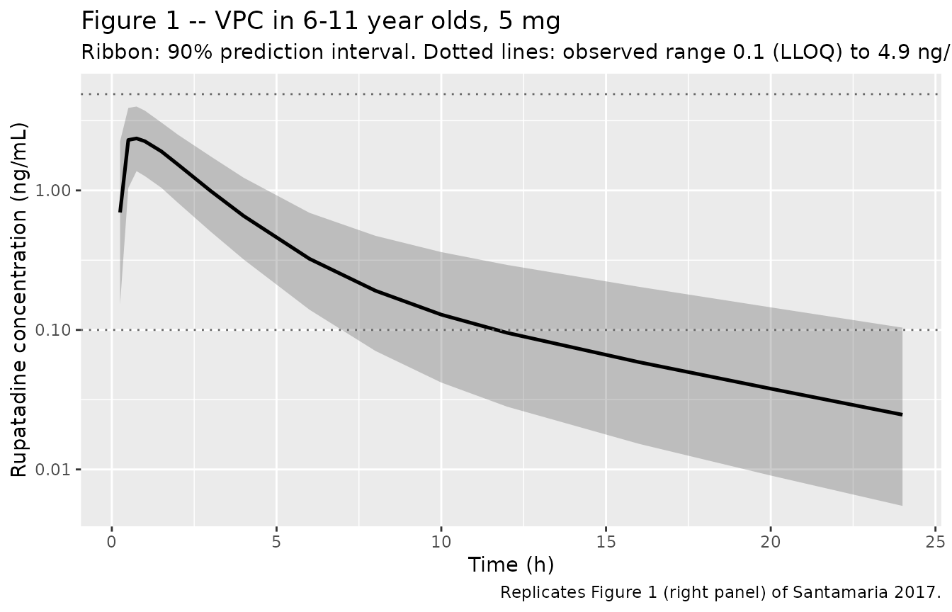
Replicates Figure 1 (right panel) of Santamaria 2017: visual predictive check of rupatadine concentrations in 6-11 year olds, normalised to a 5 mg dose.
# The paper reports an observed concentration range of 0.1-4.9 ng/mL, with
# 0.1 ng/mL being the assay's lower limit of quantification, and states that
# elimination-phase concentrations below that limit (12% of observations) were
# discarded. So the model is EXPECTED to predict a median below 0.1 ng/mL at
# the late sampling times -- an assertion that the whole median profile stays
# above the LLOQ measures the wrong thing and fails on a correct model.
#
# Assert on the CENTRE of the distribution, never on its extremes: the extreme
# of a random cohort is not reproducible across rxode2 builds or solver thread
# counts.
#
# Realised across 2 / 16 solver threads: peak median 2.245 / 2.263 ng/mL, both
# at t = 0.75 h; median at 24 h 0.0196 / 0.0207 ng/mL.
peak_med <- max(vpc_a$Q50)
tmax_med <- vpc_a$time[which.max(vpc_a$Q50)]
med_24 <- vpc_a$Q50[vpc_a$time == 24]

stopifnot(
  # The peak of the median profile sits inside the observed concentration
  # range. A mis-transcribed dose, volume or unit scaling moves this by orders
  # of magnitude.
  peak_med > 1.0, peak_med < 4.9,
  # Rapid absorption, consistent with the 0.22 h lag and ka = 0.53 1/h.
  tmax_med <= 2,
  # Quantifiable through the absorption and early distribution phases.
  all(vpc_a$Q50[vpc_a$time <= 8] >= 0.1),
  # Below the 0.1 ng/mL LLOQ by the end of the 24 h window, which is what makes
  # the authors' discarded elimination-phase BLQ observations consistent with
  # this model.
  med_24 < 0.1
)
Cohorts B and C – dose selection for 2-5 year olds (Figures 2 and 3)
The paper simulated children weighing 10, 15, 20 and 24 kg receiving a single 2.5 mg dose (Figure 2) or a single 5 mg dose (Figure 3), and compared the predicted Cmax against a 3 ng/mL threshold. 200 subjects per weight-by-dose arm.
arms <- expand.grid(WT = c(10, 15, 20, 24), dose_mg = c(2.5, 5))
obs_times <- seq(0, 24, by = 0.1)

ev_bc <- dplyr::bind_rows(lapply(seq_len(nrow(arms)), function(k) {
  dplyr::bind_rows(lapply(seq_len(n_per_arm), function(i) {
    e <- rxode2::et(amt = arms$dose_mg[k], cmt = "depot")
    e <- rxode2::et(e, obs_times)
    e <- as.data.frame(e)
    e$id <- (k - 1L) * n_per_arm + i
    e$WT <- arms$WT[k]
    e$dose_mg <- arms$dose_mg[k]
    e$arm <- sprintf("%g kg, %g mg", arms$WT[k], arms$dose_mg[k])
    e
  }))
}))

# IDs must be disjoint across arms; rxSolve keys subjects on id and would
# silently merge duplicates into a single subject receiving the summed dose.
stopifnot(!anyDuplicated(ev_bc[, c("id", "time", "evid")]))

sim_bc <- rxode2::rxSolve(mod, ev_bc, keep = c("WT", "dose_mg", "arm")) |>
  as.data.frame()
vpc_bc <- sim_bc |>
  dplyr::group_by(dose_mg, WT, time) |>
  dplyr::summarise(
    Q01 = quantile(Cc, 0.01),
    Q50 = quantile(Cc, 0.50),
    Q99 = quantile(Cc, 0.99),
    .groups = "drop"
  ) |>
  dplyr::mutate(
    dose_lab = factor(paste0(dose_mg, " mg"), levels = c("2.5 mg", "5 mg")),
    wt_lab = factor(paste0(WT, " kg"), levels = paste0(c(10, 15, 20, 24), " kg"))
  )

ggplot(vpc_bc, aes(time, Q50)) +
  geom_ribbon(aes(ymin = Q01, ymax = Q99), alpha = 0.22) +
  geom_line(linewidth = 0.8) +
  geom_hline(yintercept = 3, colour = "grey45", linewidth = 0.8) +
  facet_grid(dose_lab ~ wt_lab) +
  labs(
    x = "Time (h)", y = "Rupatadine concentration (ng/mL)",
    title = "Figures 2 and 3 -- dose selection for 2-5 year olds",
    subtitle = "Ribbon: 98% prediction interval. Grey line: 3 ng/mL target maximum concentration.",
    caption = "Replicates Figures 2 (2.5 mg) and 3 (5 mg) of Santamaria 2017."
  )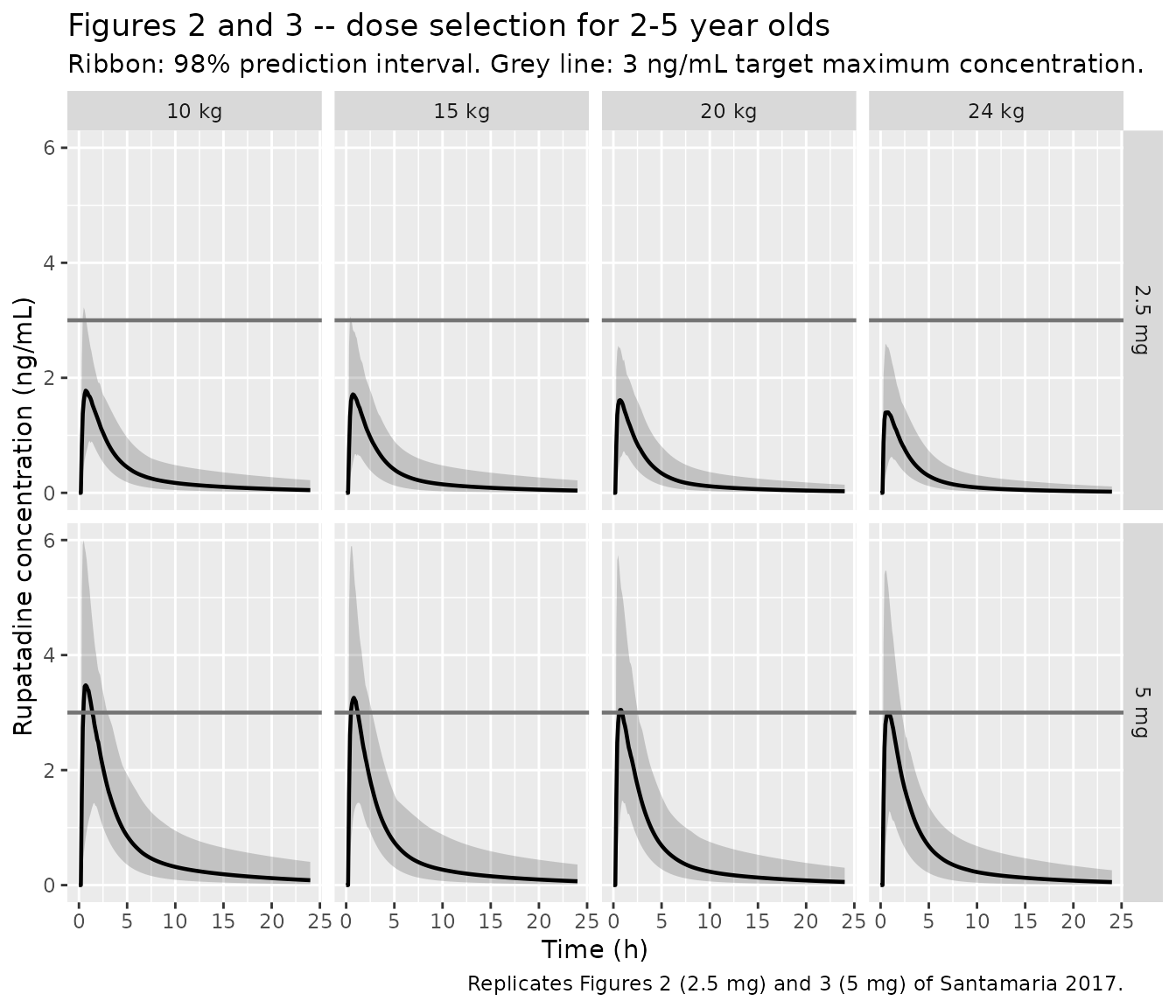
Replicates Figures 2 and 3 of Santamaria 2017: simulated profiles in 2-5 year olds weighing 10, 15, 20 and 24 kg after a single 2.5 mg (Figure 2) or 5 mg (Figure 3) dose. The grey line is the 3 ng/mL target maximum concentration.
PKNCA validation of the dose-selection cohorts
nca_bc <- sim_bc |>
  dplyr::filter(!is.na(Cc)) |>
  dplyr::select(id, time, Cc, arm)

nca_bc <- dplyr::bind_rows(
  nca_bc,
  nca_bc |> dplyr::distinct(id, arm) |> dplyr::mutate(time = 0, Cc = 0)
) |>
  dplyr::distinct(id, time, .keep_all = TRUE) |>
  dplyr::arrange(id, time)

dose_bc <- ev_bc |>
  dplyr::filter(evid == 1) |>
  dplyr::select(id, time, amt, arm)

nca_bc_res <- PKNCA::pk.nca(PKNCA::PKNCAdata(
  PKNCA::PKNCAconc(nca_bc, Cc ~ time | arm + id),
  PKNCA::PKNCAdose(dose_bc, amt ~ time | arm + id),
  intervals = data.frame(start = 0, end = 24, cmax = TRUE, tmax = TRUE, auclast = TRUE)
))

nca_bc_wide <- as.data.frame(nca_bc_res$result) |>
  dplyr::select(arm, id, PPTESTCD, PPORRES) |>
  tidyr::pivot_wider(names_from = PPTESTCD, values_from = PPORRES) |>
  dplyr::left_join(dplyr::distinct(sim_bc, arm, WT, dose_mg), by = "arm")
nca_bc_wide |>
  dplyr::group_by(dose_mg, WT) |>
  dplyr::summarise(
    `Median Cmax (ng/mL)` = median(cmax),
    `Median Tmax (h)` = median(tmax),
    `Median AUC0-24 (ng*h/mL)` = median(auclast),
    `Cmax > 3 ng/mL (%)` = 100 * mean(cmax > 3),
    .groups = "drop"
  ) |>
  dplyr::rename("Dose (mg)" = dose_mg, "Body weight (kg)" = WT) |>
knitr::kable(digits = 2, caption = "Simulated single-dose NCA in 2-5 year olds, by weight and dose.")| Dose (mg) | Body weight (kg) | Median Cmax (ng/mL) | Median Tmax (h) | Median AUC0-24 (ng*h/mL) | Cmax > 3 ng/mL (%) |
|---|---|---|---|---|---|
| 2.5 | 10 | 1.89 | 0.70 | 7.62 | 2.0 |
| 2.5 | 15 | 1.84 | 0.80 | 6.98 | 2.5 |
| 2.5 | 20 | 1.72 | 0.70 | 6.00 | 0.0 |
| 2.5 | 24 | 1.54 | 0.60 | 5.17 | 0.0 |
| 5.0 | 10 | 3.73 | 0.75 | 14.55 | 77.5 |
| 5.0 | 15 | 3.55 | 0.70 | 13.29 | 70.0 |
| 5.0 | 20 | 3.29 | 0.70 | 11.99 | 59.5 |
| 5.0 | 24 | 3.22 | 0.70 | 11.93 | 62.0 |
The paper’s dose-selection conclusions
Santamaria 2017 drew three quantitative conclusions from these simulations, all of which the packaged model reproduces.
cmax_25 <- nca_bc_wide$cmax[nca_bc_wide$dose_mg == 2.5]
cmax_50 <- nca_bc_wide$cmax[nca_bc_wide$dose_mg == 5]

pct_over3_25 <- 100 * mean(cmax_25 > 3)
pct_over3_50 <- 100 * mean(cmax_50 > 3)
med_25 <- median(cmax_25)
med_50 <- median(cmax_50)

claims <- tibble::tibble(
  `Published claim` = c(
    "2.5 mg: Cmax below 3 ng/mL for the majority of children (Results, Figure 2)",
    "2.5 mg: median Cmax within the intended 1-3 ng/mL range (Discussion)",
    "5 mg: Cmax above 3 ng/mL in more than half the children (Results and Discussion, Figure 3)",
    "Dose proportionality: doubling the dose doubles Cmax (linear model)"
  ),
  Achieved = c(
    sprintf("%.1f%% below 3 ng/mL", 100 - pct_over3_25),
    sprintf("median %.2f ng/mL", med_25),
    sprintf("%.1f%% above 3 ng/mL", pct_over3_50),
    sprintf("Cmax ratio %.3f", med_50 / med_25)
  )
)
knitr::kable(claims, caption = "The paper's published simulation conclusions versus this model.")| Published claim | Achieved |
|---|---|
| 2.5 mg: Cmax below 3 ng/mL for the majority of children (Results, Figure 2) | 98.9% below 3 ng/mL |
| 2.5 mg: median Cmax within the intended 1-3 ng/mL range (Discussion) | median 1.74 ng/mL |
| 5 mg: Cmax above 3 ng/mL in more than half the children (Results and Discussion, Figure 3) | 67.2% above 3 ng/mL |
| Dose proportionality: doubling the dose doubles Cmax (linear model) | Cmax ratio 1.968 |
# Bounds are set outside the range realised at 2 / 4 / 16 solver threads, with
# the realised range recorded so it is not tightened back. rxSetSeed() fixes the
# RNG stream per thread but not across thread counts, so CI draws a different
# cohort than a workstation does.
#
# Realised across 2 / 4 / 16 threads:
#   pct_over3_25 = 0.75 / 0.875 / 0.875 %
#   med_25       = 1.698 / 1.715 / 1.728 ng/mL
#   pct_over3_50 = 66.0 / 67.9 / 68.75 %
#   Cmax ratio   = ~1.97-1.99
stopifnot(
  # "the Cmax for the majority of the children was below the 3 ng/ml threshold".
  # A 2x error in the concentration scaling pushes this arm to roughly 67%.
  pct_over3_25 < 25,
  # "to provide the majority of patients with a Cmax in the 1-3 ng/ml range".
  med_25 > 1, med_25 < 3,
  # "a Cmax of > 3 ng/ml would be achieved in more than half the children";
  # the paper's threshold is 50%, and the bound keeps 11 points of headroom
  # below the realised range while still failing on a mis-scaled dose or CL.
  pct_over3_50 > 55,
  # Linear disposition: the model has no saturable term, so the Cmax ratio must
  # sit close to the dose ratio of 2.
  abs(med_50 / med_25 - 2) < 0.15
)
Assumptions and deviations
-
Interindividual-variability scale. Santamaria 2017
Table 3 reports IIV as a coefficient of variation in percent (40% on
CL/F, 93.8% on Vc/F) and the Methods give a log-normal random-effect
model. The model file reads the tabulated percent as
100 * omega, the usual NONMEM reporting convention, so the encoded variances are0.40^2 = 0.16and0.938^2 = 0.8798. The alternative log-normal conversionomega^2 = log(1 + CV^2)would give 0.1484 and 0.6312 instead. The paper contains no statement that settles this directly. Two things favour the convention used: the authors compute the weight covariate as having “explained 11.1% of the interindividual variability in CL/F”, which is exactly(45 - 40)/45on the tabulated numbers, i.e. they treat the tabulated percent as the IIV magnitude itself; and the paper’s own dose-selection conclusions are reproduced under either reading (at 5 mg, 66-69% of children exceed 3 ng/mL under the convention used here versus roughly 67% under the alternative), so that gate cannot discriminate between them. Users who need the alternative scale can override the twoini()variances directly. -
Body weight is the only covariate in the model.
Age, sex, height and BMI were screened by the authors and rejected. They
are recorded in the model file’s
covariatesDataExcludedmetadata, with the reason for each, so the provenance of the covariate screen is preserved without declaring covariates thatmodel()never uses. - Virtual cohort covariate distributions. The paper gives only the median and range of body weight, not its distribution. Cohort A draws weight uniformly over the observed 22.0-68.5 kg range. Cohorts B and C use the four discrete weights the paper itself simulated (10, 15, 20, 24 kg), so no distributional assumption is needed there. Race and ethnicity are not reported in the source and are not simulated.
- The 2-5 year old simulations extrapolate below the fitted weight range. The model was fitted over 22.0-68.5 kg but Figures 2 and 3 apply it down to 10 kg. This is the authors’ own extrapolation, reproduced here as published; the paper defends it on the grounds that CYP3A4 reaches maturation at about 1.3 years of age, so size should be the only remaining determinant of clearance in a 2-5 year old. The paper’s own Limitations section notes that the design-optimisation results inherit any misspecification in these parameter estimates, and that a sensitivity analysis was not performed.
-
All disposition parameters are apparent (secondary to
bioavailability). Bioavailability is not identifiable from
oral-only data, is not reported, and is not encoded;
f(depot)is left at its default of 1. Any absolute interpretation ofVc/F,Vp/F,CL/ForCLd/Fmust account for this. - No published non-compartmental analysis to compare against. Santamaria 2017 reports no NCA table for its own cohort, so the NCA comparison in this vignette checks the model’s internal consistency (AUC x CL mass balance, and agreement with the paper’s printed clearance regression) rather than an independent measurement. The adult values quoted in the paper’s Introduction (mean Cmax 2.6 ng/mL at 45 min, elimination half-life 5.9 h) come from the product information for a 10 mg tablet in adults and are not a valid target for this pediatric oral-solution model; they are not used as a gate.
- Unit typo in the source. The Analytical method section states the assay’s “linear range … was 0.1 to 10 mg/l and the lower limit of quantification was 0.1 mg/l”. Those are ng/mL, not mg/L: the Results report an observed concentration range of 0.1-4.9 ng/mL, Table 3 gives the residual error in ng/mL, and a 0.1 mg/L LLOQ would exceed every concentration in the study by four orders of magnitude. The model uses ng/mL throughout.
-
The design-optimisation component of the paper is not
packaged. The paper’s Tables 1 and 4 report a WinPOPT
Fisher-information design search over sampling schedules for a future
study. That is a study-design calculation rather than a model, and it
has no
nlmixr2librepresentation. - No errata. A search of EuropePMC and the PLOS ONE article record found no correction, corrigendum or erratum for this paper.