Meltdose tacrolimus (Kamp 2023)
Source:vignettes/articles/Kamp_2023_tacrolimus.Rmd
Kamp_2023_tacrolimus.RmdModel and source
- Citation: Kamp J, Zwart TC, Meziyerh S, van der Boog PJM, Nijgh EE, van Duin K, de Vries APJ, Moes DJAR. Meltdose Tacrolimus Population Pharmacokinetics and Limited Sampling Strategy Evaluation in Elderly Kidney Transplant Recipients. Pharmaceutics. 2024;16(1):17. doi:10.3390/pharmaceutics16010017. Published online 21 December 2023; PMCID PMC10819724. Structural model, final parameter estimates and the NONMEM control stream are taken from Table 2 and Supplementary Data S1.
- Description: Two-compartment population PK model for meltdose (LCP, prolonged-release) tacrolimus in elderly de novo kidney transplant recipients. Oral absorption is a chain of three first-order compartments (the dosing depot plus two absorption transit compartments) sharing a single transit rate constant Ktr, feeding a two-compartment disposition with linear elimination. Apparent oral bioavailability is fixed at 1, so CL, Q, Vc and Vp are apparent (/F) values. The peripheral volume is fixed at 500 L per 70 kg because it was not identifiable. Absorption lag time follows a two-class latent mixture gated by MIX_LAGGED_ABS: the lagged class (74% of the population) carries a 2.29 h lag and the no-lag class (26%) carries none. Allometric scaling on body weight (exponent 0.75 on CL and Q, 1 on Vc and Vp, reference 70 kg) was included a priori; no clinical covariate was retained in the final model. Inter-individual variability is log-normal on Ktr and on a correlated CL/Vc block; inter-occasion variability is carried on CL across five occasions. The proportional residual error switches per observation between whole blood (venous) and dried blood spot (capillary) sampling.
- Article: https://doi.org/10.3390/pharmaceutics16010017
- Supplement (figures S1-S6, tables S1-S3 and the NONMEM control stream, Supplementary Data S1): https://www.mdpi.com/article/10.3390/pharmaceutics16010017/s1
Meltdose tacrolimus (Envarsus) is a prolonged-release oral formulation. Kamp 2023 developed a population PK model for it in elderly de novo kidney transplant recipients, then used the model to derive limited sampling strategies for AUC estimation and to quantify how long meltdose tacrolimus takes to reach steady state.
Population
Thirty-four de novo kidney transplant recipients aged 65 years or older were analysed (36 enrolled, 2 excluded after their transplantation was postponed). Median age was 71.5 years (IQR 68.8-73.2) and median weight 77.0 kg (IQR 68.1-84.5); 12 (35.3%) were female. All patients started on meltdose tacrolimus 7 mg once daily on the day of transplantation, with subsequent AUC-guided dose individualisation; the median dose at AUC sampling was 6.0 mg (IQR 3.25-7.0). CYP3A5 genotype was 3/3 in 26 (76.5%), 1/3 in 6 (17.6%) and 1/1 in 2 (5.9%). The dataset comprised 546 concentrations over 87 AUC profiles (median 2 per subject, range 1-5); 37 of those profiles (42.5%) were abbreviated dried blood spot profiles collected at home by 20 (58.8%) of the patients. Baseline characteristics are Kamp 2023 Table 1.
The same information is available programmatically from the model’s
population metadata:
str(rxode2::rxode(readModelDb("Kamp_2023_tacrolimus"))$population)
#> ℹ parameter labels from comments will be replaced by 'label()'
#> Warning: some etas defaulted to non-mu referenced, possible parsing error: etaiov_cl_1, etaiov_cl_2, etaiov_cl_3, etaiov_cl_4, etaiov_cl_5
#> as a work-around try putting the mu-referenced expression on a simple line
#> List of 15
#>  $ species       : chr "human"
#>  $ n_subjects    : int 34
#>  $ n_studies     : int 1
#>  $ age_range     : chr ">= 65 years at transplantation"
#>  $ age_median    : chr "71.5 years (IQR 68.8-73.2)"
#>  $ weight_median : chr "77.0 kg (IQR 68.1-84.5)"
#>  $ sex_female_pct: num 35.3
#>  $ disease_state : chr "de novo kidney transplant recipients aged 65 years or older, on a tacrolimus / mycophenolate / prednisolone or "| __truncated__
#>  $ dose_range    : chr "Meltdose tacrolimus (Envarsus) 7 mg once daily from the day of transplantation, subsequently individualised by "| __truncated__
#>  $ regions       : chr "Netherlands (Leiden University Medical Center)"
#>  $ genotype      : chr "CYP3A5*3/*3 non-expressers 26 (76.5%), CYP3A5*1/*3 6 (17.6%), CYP3A5*1/*1 2 (5.9%)"
#>  $ renal_function: chr "Serum creatinine median 132 umol/L (IQR 99-177) at AUC sampling"
#>  $ co_medication : chr "Mycophenolate mofetil 500 mg b.i.d.; prednisolone 50 mg b.i.d. tapered to 25 mg b.i.d. at day 4, 10 mg q.d. aft"| __truncated__
#>  $ n_observations: chr "546 tacrolimus concentrations over 87 AUC profiles (median 2 per subject, range 1-5); 37 of the AUCs (42.5%) we"| __truncated__
#>  $ notes         : chr "Add-on pharmacokinetic study to the OPTIMIZE trial (NCT03497196) at the Leiden University Medical Center site. "| __truncated__
Source trace
Per-parameter provenance is recorded as an in-file comment beside
each ini() entry in
inst/modeldb/specificDrugs/Kamp_2023_tacrolimus.R.
Collected here for review. “S1” is Supplementary Data S1, the paper’s
NONMEM control stream.
| Equation / parameter | Value | Source location |
|---|---|---|
lktr (Ktr) |
0.752 1/h | Table 2 “Ktr (h-1)”, RSE 21%; S1 $THETA(6)
|
ltlag (lag, lagged class) |
2.29 h | Table 2 “Lag (h)”, RSE 2%; S1 $THETA(5)
|
lcl (CL/F at 70 kg) |
19.6 L/h | Table 2 “CL/F”, RSE 8%; S1 $THETA(7)
|
lvc (Vc/F at 70 kg) |
123 L | Table 2 “Vc/F”, RSE 38%; S1 $THETA(8)
|
lq (Q/F at 70 kg) |
74.9 L/h | Table 2 “Q/F”, RSE 9%; S1 $THETA(9)
|
lvp (Vp/F at 70 kg) |
500 L, fixed | Table 2 “Vp/F (Fixed)”; Sect. 3.3.1 (not identifiable; fixed to the
literature values of Kamp refs [10] Martial 2021 and [20] Benkali 2010);
S1 $THETA(10) 500 FIX
|
lfdepot (F) |
1, fixed | Table 2 “F (Fixed)”; Sect. 2.3.1 |
e_wt_cl_q |
0.75, fixed | Sect. 2.3.2 allometric equation; S1
ALLO_CL = ALLO_V ** 0.75
|
e_wt_vc_vp |
1, fixed | Sect. 2.3.2 allometric equation; S1 ALLO_V = WT/70
|
| mixture proportion (no-lag class) | 26% | Table 2 “Pop parameter (%)”, RSE 50%; S1 $THETA(11)
(see Assumptions) |
etalktr |
0.312 | S1 $OMEGA; Table 2 IIV Ka 60.5% CV = sqrt(exp(0.312) -
1) |
etalcl |
0.0979 | S1 $OMEGA BLOCK(2); Table 2 IIV CL 32.1% CV |
cov(etalcl, etalvc) |
0.23 | S1 $OMEGA BLOCK(2); correlation 0.23/sqrt(0.0979*0.609)
= 0.94, quoted as “94% covariance” in Sect. 3.3.1 |
etalvc |
0.609 | S1 $OMEGA BLOCK(2); Table 2 IIV Vc 91.6% CV |
etaiov_cl_1 .. etaiov_cl_5
|
0.224 | S1 $OMEGA BLOCK(1) + 4 x SAME; Table 2 IOV
CL 50.1% CV |
propSdVenous |
0.208 | Table 2 “Proportional Error Whole blood”, RSE 8%; S1
$THETA(1)
|
propSdCapillary |
0.307 | Table 2 “DBS”, RSE 12%; S1 $THETA(2)
|
addSd |
1e-4 ug/L, fixed | S1 $THETA(3) 0.0001 FIX (numerical stabiliser; not in
Table 2) |
ODE chain
depot -> transit1 -> transit2 -> central at
ktr
|
n/a | S1 $MODEL / $DES; Figure 2 |
central <-> peripheral1 via
k12/k21
|
n/a | S1 $PK K45 = Q/V2,
K54 = Q/V3
|
alag(depot) <- tlag * MIX_LAGGED_ABS |
n/a | S1 $MIX / $PK ALAG1; Sect.
3.3.1 |
Cc <- 1000 * central / vc |
n/a | S1 $PK S4 = V2/1000 (mg and L in, ug/L
out) |
| per-record residual switch | n/a | S1 $ERROR IF(DBS0.EQ.1); Sect. 3.3.1 |
The final model retained no clinical covariate.
Hematocrit and CYP3A5 genotype were selected by the stepwise search but
rejected as clinically irrelevant (Sect. 3.3.2); they are documented in
the model file’s covariatesDataExcluded metadata together
with age, sex, prednisolone dose, calcium-channel-blocker use and
diabetes.
Virtual cohort
Original observed data are not publicly available. The cohort below mirrors the simulation Kamp 2023 itself ran for its time-to-steady-state analysis (Sect. 2.3.4): a 70 kg individual receiving 7 mg meltdose tacrolimus once daily, followed for 14 days. The paper simulated 1000 profiles; 200 is used here (the per-arm cap for these vignettes) and is ample for the median and quartile summaries the paper reports.
# `set.seed()` seeds R's RNG (used for the Bernoulli mixture draw below). It
# does NOT seed rxode2's simulation RNG, whose streams are partitioned per
# solver thread -- so this cohort differs between a 2-core CI runner and a
# 16-thread workstation. Every assertion below is written to hold for any
# cohort the model can produce.
set.seed(2024)

n_sub  <- 200L
tau    <- 24      # dosing interval (h)
n_dose <- 14L     # 14 daily doses -> the paper's day-14 steady-state anchor
t_end  <- tau * n_dose

subjects <- tibble(
  id = seq_len(n_sub),
  WT = 70,
  OCC = 1L,
  # The lagged class is the 74% majority; see "Assumptions and deviations".
  MIX_LAGGED_ABS = rbinom(n_sub, 1L, 0.74),
  SAMPLE_CAPILLARY = 0L
)

# Hourly over the whole course, refined to 15 min over the first and last
# dosing intervals, which are the two windows any Cmax / Tmax is read from.
obs_times <- sort(unique(c(
  seq(0, t_end, by = 1),
  seq(0, tau, by = 0.25),
  seq(t_end - tau, t_end, by = 0.25)
)))

events <- rxode2::et(amt = 7, ii = tau, addl = n_dose - 1L, cmt = "depot") |>
  rxode2::et(obs_times) |>
  rxode2::et(id = seq_len(n_sub)) |>
  as.data.frame() |>
  dplyr::left_join(subjects, by = "id")

stopifnot(!anyDuplicated(unique(events[, c("id", "time", "evid")])))

# Realised share of the lagged absorption class (target 74%).
sprintf("%.0f%% of the cohort drew the lagged-absorption class",
        100 * mean(subjects$MIX_LAGGED_ABS))
#> [1] "74% of the cohort drew the lagged-absorption class"
Simulation
mod <- readModelDb("Kamp_2023_tacrolimus")
sim <- rxode2::rxSolve(
  mod, events = events,
  maxsteps = 200000L,          # 14 lagged daily doses exhaust the default
  addDosing = FALSE,
  keep = c("MIX_LAGGED_ABS")
) |>
  as.data.frame()
#> ℹ parameter labels from comments will be replaced by 'label()'
#> Warning: some etas defaulted to non-mu referenced, possible parsing error: etaiov_cl_1, etaiov_cl_2, etaiov_cl_3, etaiov_cl_4, etaiov_cl_5
#> as a work-around try putting the mu-referenced expression on a simple line
Replicate Figure 4C: median concentration-time profile
# Replicates Figure 4C of Kamp 2023: median simulated tacrolimus
# concentration (IQR shaded) vs. time after tacrolimus initiation, 70 kg
# individual on 7 mg meltdose tacrolimus q.d.
prof <- sim |>
  group_by(time) |>
  summarise(
    Q25 = quantile(Cc, 0.25),
    Q50 = median(Cc),
    Q75 = quantile(Cc, 0.75),
    .groups = "drop"
  )

ggplot(prof, aes(time, Q50)) +
  geom_ribbon(aes(ymin = Q25, ymax = Q75), fill = "grey70", alpha = 0.5) +
  geom_line(linewidth = 0.4) +
  scale_x_continuous(breaks = seq(0, t_end, by = 48)) +
  labs(x = "Time after tacrolimus initiation (h)",
       y = "Tacrolimus concentration (ug/L)",
       caption = "Replicates Figure 4C of Kamp 2023.")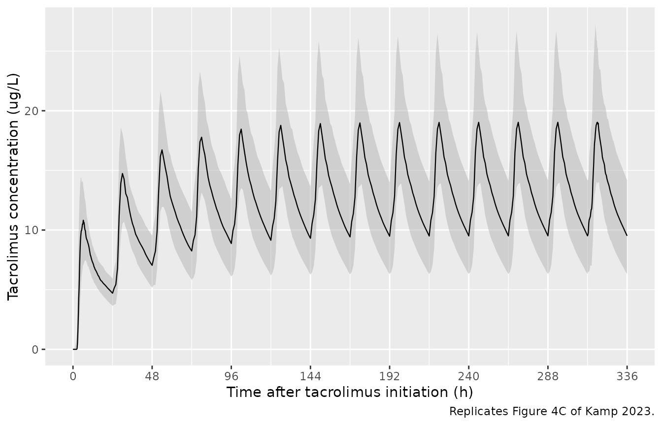
The published panel rises to a first-dose median peak just above 11 ug/L, accumulates over roughly the first week, and settles into a steady-state interval whose nadir sits a few hours after each dose – the visible signature of the absorption lag – before rising to a peak near 20 ug/L.
day1 <- prof |> filter(time <= tau)
ss   <- prof |> filter(time >= t_end - tau, time <= t_end)

fig4c <- tibble(
  quantity = c("Day-1 median Tmax (h)", "Day-1 median Cmax (ug/L)",
               "Steady-state median peak (ug/L)",
               "Steady-state median nadir (ug/L)"),
  simulated = c(day1$time[which.max(day1$Q50)], max(day1$Q50),
                max(ss$Q50), min(ss$Q50)),
  # On-screen digitisation of the published panel (see Assumptions). The
  # x-axis resolves ~2 pixels per hour, so times carry about +/- 0.5 h and
  # concentrations a few percent of systematic y-calibration error.
  figure_4c = c(6.08, 11.27, 20.55, 10.27)
)
fig4c |>
  dplyr::rename("Quantity" = quantity,
                "Simulated" = simulated,
                "Figure 4C (digitised)" = figure_4c) |>
  knitr::kable(digits = 2,
               caption = paste("Figure 4C reference values are read off the",
                               "published panel by on-screen digitisation and",
"are approximate (see Assumptions)."))| Quantity | Simulated | Figure 4C (digitised) |
|---|---|---|
| Day-1 median Tmax (h) | 6.25 | 6.08 |
| Day-1 median Cmax (ug/L) | 10.82 | 11.27 |
| Steady-state median peak (ug/L) | 19.03 | 20.55 |
| Steady-state median nadir (ug/L) | 9.51 | 10.27 |
# The three concentrations landed +11 / +10 / +8% against the digitised panel
# in one cohort and -4 / -7 / -7% in another, so the gap is cohort redraw
# rather than a systematic offset in either direction. 30% is roughly 3x the
# largest deviation seen and still goes red on a mis-transcribed clearance,
# dose or scale factor, each of which moves these by tens of percent.
stopifnot(max(abs(fig4c$simulated[2:4] / fig4c$figure_4c[2:4] - 1)) < 0.30)

# Tmax is the one quantity that discriminates the two readings of the
# absorption-lag mixture (see Assumptions): 6.0 h under the adopted
# 74%-lagged reading vs 4.25 h under the alternative. 1.5 h keeps the gate
# able to detect that flip while admitting the cohort-to-cohort wobble of a
# 200-subject median read on a 15-minute grid.
stopifnot(abs(fig4c$simulated[1] - fig4c$figure_4c[1]) < 1.5)
Replicate Figure 4A/B: time to steady state
Kamp 2023 Sect. 2.3.4 defines the fraction of steady state as
FSS = IPRED / Ctrough_14 * 100, where
Ctrough_14 is the trough concentration on day 14, and
evaluates it at the daily troughs. The reported results (Sect. 3.3.4)
are a median time to 90% of steady state of 96 h (IQR 72-120) and to 97%
of 144 h (IQR 120-312), with 76% / 40% of subjects at 90% / 97% of
steady state five days after initiation and 94% / 71% after seven
days.
troughs <- sim |>
  filter(time %in% seq(tau, t_end, by = tau)) |>
  select(id, time, Cc) |>
  group_by(id) |>
  mutate(fss = 100 * Cc / Cc[time == t_end]) |>
  ungroup()

first_time_at <- function(threshold) {
  troughs |>
    filter(fss >= threshold) |>
    group_by(id) |>
    summarise(t = min(time), .groups = "drop")
}
t90 <- first_time_at(90)
t97 <- first_time_at(97)

prob_at <- function(threshold, when) {
  100 * mean(troughs$fss[troughs$time == when] >= threshold)
}

ss_tab <- tibble(
  claim = c("Median time to 90% of steady state (h)",
            "Median time to 97% of steady state (h)",
            "P(>= 90% of steady state) at day 5 (%)",
            "P(>= 97% of steady state) at day 5 (%)",
            "P(>= 90% of steady state) at day 7 (%)",
            "P(>= 97% of steady state) at day 7 (%)"),
  published = c(96, 144, 76, 40, 94, 71),
  simulated = c(median(t90$t), median(t97$t),
                prob_at(90, 120), prob_at(97, 120),
                prob_at(90, 168), prob_at(97, 168))
)
ss_tab |>
  dplyr::rename("Claim" = claim,
                "Published (Kamp 2023)" = published,
                "Simulated" = simulated) |>
  knitr::kable(digits = 1,
caption = "Time to steady state: Kamp 2023 Sect. 3.3.4 vs. simulation.")| Claim | Published (Kamp 2023) | Simulated |
|---|---|---|
| Median time to 90% of steady state (h) | 96 | 96.0 |
| Median time to 97% of steady state (h) | 144 | 144.0 |
| P(>= 90% of steady state) at day 5 (%) | 76 | 83.0 |
| P(>= 97% of steady state) at day 5 (%) | 40 | 45.5 |
| P(>= 90% of steady state) at day 7 (%) | 94 | 95.5 |
| P(>= 97% of steady state) at day 7 (%) | 71 | 79.0 |
# The two medians are read off a 24-h grid, so they can only land on a
# multiple of 24; one grid step either side is the tightest bound that can
# hold across cohorts.
stopifnot(
  abs(ss_tab$simulated[1] - 96)  <= 24,
  abs(ss_tab$simulated[2] - 144) <= 48
)
# The four probabilities are cohort proportions, and they move noticeably
# between cohorts: the largest gap to a published value was 2 points in one
# 200-subject draw and 8 points in another. The binomial standard error at
# n = 200 near p = 0.4 is about 3.5 points, and Kamp 2023 simulated 1000
# subjects, so some of that gap is irreducible. 12 points sits outside the
# observed range with headroom and still goes red on a structural error (a
# wrong CL or Vp moves these by 30 points or more). Do not tighten this to
# whatever a single local run happens to give.
stopifnot(max(abs(ss_tab$simulated[3:6] - ss_tab$published[3:6])) < 12)
# Replicates Figure 4B of Kamp 2023: probability of having reached at least
# 90% (blue) and 97% (black) of the steady-state concentration.
troughs |>
  group_by(time) |>
  summarise(`90%` = 100 * mean(fss >= 90),
            `97%` = 100 * mean(fss >= 97), .groups = "drop") |>
  pivot_longer(-time, names_to = "threshold", values_to = "probability") |>
  ggplot(aes(time, probability, colour = threshold)) +
  geom_step(linewidth = 0.6) +
  scale_x_continuous(breaks = seq(0, t_end, by = 48)) +
  scale_colour_manual(values = c(`90%` = "#2C7FB8", `97%` = "black")) +
  labs(x = "Time after tacrolimus initiation (h)",
       y = "Steady state probability (%)", colour = "Fraction of\nsteady state",
       caption = "Replicates Figure 4B of Kamp 2023.")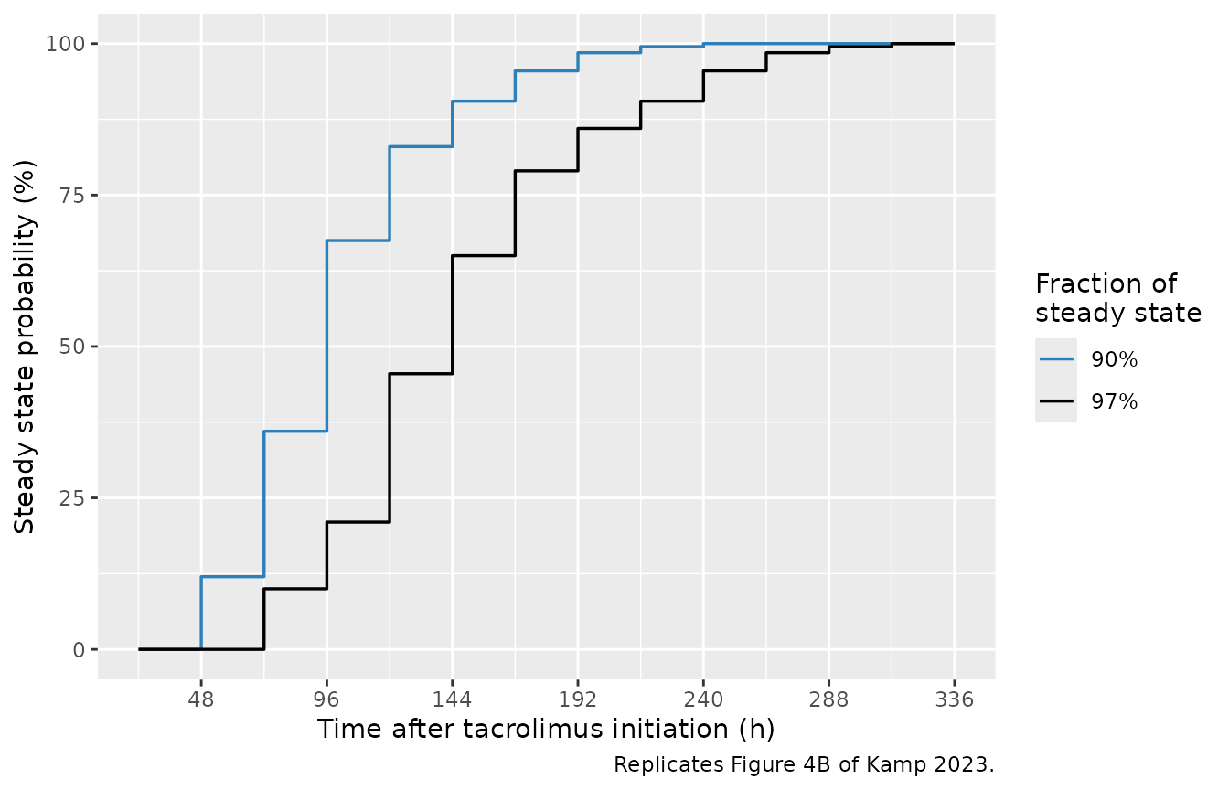
PKNCA validation
Kamp 2023 has no published NCA table. It does, however, define a reference exposure used throughout the paper (Sect. 2.3.1 and 2.3.3, and the captions of Figures S3 and S4):
AUC0-24 = (F x D x 1000) / CL, with F fixed at 1, D the
dose in mg and CL the apparent elimination clearance in L/h.
That identity is the yardstick every limited sampling strategy in the
paper was scored against, so reproducing it from a trapezoidal NCA of
the simulated steady-state interval is a direct check of the absorption
chain’s mass balance, the bioavailability anchor and the
S4 = Vc/1000 concentration scaling. It is evaluated at
typical values (random effects zeroed) so the published CL of 19.6 L/h
at 70 kg applies exactly, across the cohort’s median dose and its
interquartile dose range (Table 1).
doses <- c(3.25, 6.0, 7.0)

make_dose_arm <- function(i) {
  rxode2::et(amt = doses[i], ii = tau, addl = n_dose - 1L, cmt = "depot") |>
    rxode2::et(seq(0, t_end, by = 0.25)) |>
    as.data.frame() |>
    mutate(id = i, WT = 70, OCC = 1L, MIX_LAGGED_ABS = 1L,
           SAMPLE_CAPILLARY = 0L,
           treatment = sprintf("%.2f mg q.d.", doses[i]))
}
events_tv <- bind_rows(lapply(seq_along(doses), make_dose_arm))
stopifnot(!anyDuplicated(unique(events_tv[, c("id", "time", "evid")])))

sim_tv <- rxode2::rxSolve(
  rxode2::zeroRe(rxode2::rxode(mod)), events = events_tv,
  maxsteps = 200000L, addDosing = FALSE, keep = c("treatment")
) |>
  as.data.frame()
#> ℹ parameter labels from comments will be replaced by 'label()'
#> Warning: some etas defaulted to non-mu referenced, possible parsing error: etaiov_cl_1, etaiov_cl_2, etaiov_cl_3, etaiov_cl_4, etaiov_cl_5
#> as a work-around try putting the mu-referenced expression on a simple line
#> Warning: some etas defaulted to non-mu referenced, possible parsing error: etaiov_cl_1, etaiov_cl_2, etaiov_cl_3, etaiov_cl_4, etaiov_cl_5
#> as a work-around try putting the mu-referenced expression on a simple line
#> ℹ omega/sigma items treated as zero: 'etalktr', 'etalcl', 'etalvc', 'etaiov_cl_1', 'etaiov_cl_2', 'etaiov_cl_3', 'etaiov_cl_4', 'etaiov_cl_5'
#> Warning: multi-subject simulation without without 'omega'

# Restrict to the final dosing interval; the interval start is a real
# measurement, so no time-zero back-fill is needed here.
sim_nca <- sim_tv |>
  dplyr::filter(!is.na(Cc), time >= t_end - tau) |>
  dplyr::select(id, time, Cc, treatment)
stopifnot(nrow(sim_nca) > 0)

dose_df <- events_tv |>
  dplyr::filter(evid == 1) |>
  dplyr::group_by(id, treatment) |>
  dplyr::summarise(time = max(time), amt = dplyr::first(amt), .groups = "drop") |>
  dplyr::select(id, time, amt, treatment)

conc_obj <- PKNCA::PKNCAconc(sim_nca, Cc ~ time | treatment + id,
                             concu = "ug/L", timeu = "h")
dose_obj <- PKNCA::PKNCAdose(dose_df, amt ~ time | treatment + id,
                             doseu = "mg")

intervals <- data.frame(
  start   = t_end - tau,
  end     = t_end,
  cmax    = TRUE,
  tmax    = TRUE,
  cmin    = TRUE,
  auclast = TRUE
)
nca_res <- PKNCA::pk.nca(PKNCA::PKNCAdata(conc_obj, dose_obj,
                                          intervals = intervals))
Comparison against the paper’s reference AUC
published <- tibble::tibble(
  treatment  = sprintf("%.2f mg q.d.", doses),
  # Kamp 2023 AUCref = (F * D * 1000) / CL with F = 1 and CL = 19.6 L/h at 70 kg.
  auclast    = doses * 1000 / 19.6
)

cmp <- nlmixr2lib::ncaComparisonTable(
  simulated     = nca_res,
  reference     = published,
  by            = "treatment",
  units         = c(auclast = "ug*h/L"),
  tolerance_pct = 20
)
knitr::kable(cmp, caption = paste(
  "Simulated steady-state AUC0-24 vs. the paper's reference AUC identity",
  "(F x D x 1000) / CL. * differs from reference by >20%."
))| NCA parameter | treatment | Reference | Simulated | % diff |
|---|---|---|---|---|
| AUClast (ug*h/L) | 3.25 mg q.d. | 166 | 166 | -0.0% |
| AUClast (ug*h/L) | 6.00 mg q.d. | 306 | 306 | -0.0% |
| AUClast (ug*h/L) | 7.00 mg q.d. | 357 | 357 | -0.0% |
auc_sim <- as.data.frame(nca_res$result) |>
  filter(PPTESTCD == "auclast") |>
  left_join(published, by = "treatment", suffix = c("", "_ref"))
pct <- 100 * (auc_sim$PPORRES / auc_sim$auclast - 1)

# Deterministic (typical-value) comparison: the only error left is the
# trapezoidal discretisation of a 0.25 h grid, so a tight bound is correct
# here and is what makes this gate useful. Realised 0.014% at every dose.
stopifnot(max(abs(pct)) < 0.5)

# Dose proportionality: AUCref is linear in dose, and so is the model.
ratio <- auc_sim$PPORRES / doses
stopifnot(max(ratio) / min(ratio) - 1 < 0.01)
Steady-state Tmax and Cmin from the same
NCA give the other two readable features of Figure 4C:
# PKNCA already reports tmax relative to the start of the interval, so it
# reads directly as hours after the 14th dose.
as.data.frame(nca_res$result) |>
  filter(PPTESTCD %in% c("cmax", "tmax", "cmin")) |>
  select(treatment, PPTESTCD, PPORRES) |>
  pivot_wider(names_from = PPTESTCD, values_from = PPORRES) |>
  rename("Dose group" = treatment,
         "Cmax,ss (ug/L)" = cmax,
         "Tmax,ss (h post dose)" = tmax,
         "Cmin,ss (ug/L)" = cmin) |>
  knitr::kable(digits = 2,
caption = "Typical-value steady-state NCA over the 14th dosing interval.")| Dose group | Cmax,ss (ug/L) | Cmin,ss (ug/L) | Tmax,ss (h post dose) |
|---|---|---|---|
| 3.25 mg q.d. | 10.75 | 4.64 | 6.75 |
| 6.00 mg q.d. | 19.85 | 8.56 | 6.75 |
| 7.00 mg q.d. | 23.16 | 9.99 | 6.75 |
Assumptions and deviations
-
Direction of the absorption-lag mixture (the one substantive judgement in this extraction). Kamp 2023’s source is self-contradictory about which class the estimated mixture proportion of 26% belongs to.
- Table 2 and Table S2 footnote the parameter as “Pop parameter,
proportion of the population belonging to the group
without oral lag time”, and the
$THETAcomments in Supplementary Data S1 agree with that reading (0 FIX ; Absorption lag time for group 1, withP(1) = THETA(11) = 0.26). Under this reading 74% of subjects carry the 2.29 h lag. - The
$PKblock printed in the same supplement readsIF(MIXNUM.EQ.2) ALAG1 = THETA(4) ELSE ALAG1 = THETA(5), which assigns the 2.29 h lag toMIXNUM = 1and therefore to the 26% probability – the opposite assignment, and inconsistent with its own$THETAcomments.
The footnote reading (74% lagged) is adopted, on the evidence of the paper’s own Figure 4C. That panel is the median of 1000 profiles simulated from this final model for a 70 kg subject on 7 mg q.d., so it is a direct readout of the fitted mixture. Its median sits on the baseline for the first three hours and peaks at about 6.1 h (on-screen digitisation of the published panel; the x-axis resolution is roughly 2 pixels per hour, so treat this as +/- 0.5 h). Simulating both readings gives a day-1 median Tmax of 6.0-6.25 h under the 74%-lagged reading, versus 4.25 h under the 26%-lagged reading – the latter also puts the median at 5.4 ug/L by 2 h, where the published panel is still flat on zero. A majority-lagged population is additionally what makes the median profile show a lag at all: with only 26% lagged, the median subject has none, and the published panel would not show the flat first three hours or the post-dose nadir that it does.
The consequence of getting this wrong is a roughly 2 h shift in Tmax and no change to AUC, so the steady-state and exposure checks above cannot discriminate the two readings – only the shape checks can. Both the model file’s
covariateData[[MIX_LAGGED_ABS]]$notesand theMIX_LAGGED_ABSentry ininst/references/covariate-columns.mdrecord the discrepancy so a future reader is not surprised by the supplement. - Table 2 and Table S2 footnote the parameter as “Pop parameter,
proportion of the population belonging to the group
without oral lag time”, and the
The mixture proportion is metadata, not a parameter. Following the convention set by
Bonate_2004_apomineandFrymoyer_2013_mycophenolic_acid, class membership enters as the binaryMIX_LAGGED_ABScovariate and the 26% / 74% split is documented rather than estimated. To simulate a population, drawMIX_LAGGED_ABS ~ Bernoulli(0.74)per subject as the cohort chunk above does; for a typical-value profile, set it to 1.Figure 4C reference values are digitised, not published. The four numbers in the Figure 4C comparison table (Tmax, Cmax, steady-state peak and trough) were read off the published panel by on-screen digitisation; Kamp 2023 prints none of them. They are used only as loose shape checks, with bounds set well outside the digitisation error. Every gate that uses a printed value – the six time-to-steady-state claims and the reference AUC identity – is tighter.
Occasion is held at 1. The model carries five inter-occasion variability slots on CL because the paper’s dataset had up to five AUC profiles per patient. Forward simulations of a single continuous treatment course have no natural occasion boundary, so
OCC = 1is used throughout and the IOV contributes one draw per subject rather than switching mid-course. SetOCCto 1-5 per profile to reproduce the paper’s within-subject occasion-to-occasion variability; values outside 1-5 switch all IOV indicators off and leave only the IIV.The limited sampling strategies are not reproduced. Table S3 and the paper’s LSS conclusions (best three-sample scheme T = 0, 2, 6 h; best four-sample schemes T = 0, 2, 6, 8 h and T = 0, 1, 6, 8 h) come from maximum-a-posteriori Bayesian re-estimation of each simulated subject from a reduced sampling schedule. That is a fitting exercise rather than a simulation, and is outside what a packaged model plus a validation vignette can check. The structural model that the LSS analysis rests on is what is validated here.
The alternative covariate model is not encoded. Table S2 reports a second parameter set including hematocrit (-4.94) and CYP3A5 expresser (0.625) effects on CL. Kamp 2023 rejected both as clinically irrelevant (Sect. 3.3.2) and reports the covariate-free model as final, so the final model is what is packaged. The screened covariates are recorded in the model file’s
covariatesDataExcludedmetadata.Whole blood is the reference matrix.
SAMPLE_CAPILLARY = 0is used throughout, which selects the 20.8% whole-blood proportional residual error. Set it to 1 on records collected as dried blood spots to select the 30.7% term. The choice affects only the residual error, never the structural prediction: Kamp 2023 modelled DBS and whole blood as measurements of the same underlying concentration differing in precision. The switch is written arithmetically insidemodel()(propSd <- propSdCapillary * SAMPLE_CAPILLARY + propSdVenous * (1 - SAMPLE_CAPILLARY)), following theSAMPLE_CAPILLARYregister entry and its founding exampleCleary_2023_risdiplam.The additive residual term is a stabiliser.
addSdis fixed at 1e-4 ug/L, matching$THETA(3) 0.0001 FIXin the control stream, where it exists only to keep the residual weight away from zero. It is not reported in Table 2 and is numerically irrelevant on a ug/L scale.Fitting-dataset profiles were not all at steady state. The first AUC was obtained a median of 7 days after transplantation, and the paper’s own analysis concludes that 5-7 days are needed to reach 90% of steady state. The model was fitted to the full time course rather than to steady-state profiles, so it is appropriate for de novo dosing simulations from day 0 – which is how it is used above.