Mouse brain-ECF PK with LeiCNS-PK3.0, 10 drugs (Saleh 2023)
Source:vignettes/articles/Saleh_2023_leicns_pk30_mouse_brain.Rmd
Saleh_2023_leicns_pk30_mouse_brain.RmdModel and source
- Citation: Saleh MAA, Gulave B, Campagne O, Stewart CF, Elassaiss-Schaap J, de Lange ECM. Using the LeiCNS-PK3.0 Physiologically-Based Pharmacokinetic Model to Predict Brain Extracellular Fluid Pharmacokinetics in Mice. Pharm Res. 2023;40(11):2555-2566. doi:[10.1007/s11095-023-03554-5](https://doi.org/10.1007/s11095-023-03554-5).
- Upstream structural source: Saleh MAA et al. J Pharmacokinet
Pharmacodyn. 2021;48(5):725-741. doi:[10.1007/s10928-021-09768-7](https://doi.org/10.1007/s10928-021-09768-7) (reference
[13] of the 2023 paper). The 2023 paper prints no equations at
all – it cites the LeiCNS-PK3.0 structure to this predecessor.
The supplementary equations of the 2021 paper (aqueous diffusivity
Daq, passive permeabilityP0, paracellular / transcellular barrier clearancesQp/Qt, and the asymmetry-factor closed forms) and its Supplementary Figure 1 (the fully labelled topology) are what make this extraction possible.
Saleh 2023 is a mouse re-parameterisation of the previously published rat / human LeiCNS-PK3.0 CNS PBPK model. No CNS parameter was estimated: every value is either mouse physiology collected from the literature (Table III) or derived from the drug’s physicochemical properties (Table I). The paper evaluates the resulting data-independent predictions of unbound brain extracellular fluid (brain ECF) concentrations against microdialysis data for 10 drugs.
Ten model files are packaged, one per drug, because each drug carries its own empirical plasma PK model, its own route of administration and its own drug-specific CNS parameter set:
drugs <- c("cyclophosphamide", "quinidine", "erlotinib", "phenobarbital",
           "colchicine", "ribociclib", "topotecan", "cefadroxil",
           "prexasertib", "methotrexate")
models <- paste0("Saleh_2023_", drugs, "_mouse_pbpk")
models
#>  [1] "Saleh_2023_cyclophosphamide_mouse_pbpk"
#>  [2] "Saleh_2023_quinidine_mouse_pbpk"
#>  [3] "Saleh_2023_erlotinib_mouse_pbpk"
#>  [4] "Saleh_2023_phenobarbital_mouse_pbpk"
#>  [5] "Saleh_2023_colchicine_mouse_pbpk"
#>  [6] "Saleh_2023_ribociclib_mouse_pbpk"
#>  [7] "Saleh_2023_topotecan_mouse_pbpk"
#>  [8] "Saleh_2023_cefadroxil_mouse_pbpk"
#>  [9] "Saleh_2023_prexasertib_mouse_pbpk"
#> [10] "Saleh_2023_methotrexate_mouse_pbpk"
CNS structure
Nine CNS compartments, driven by the empirical plasma model as a forcing function (brain uptake does not deplete plasma – this is how the paper is published, so the plasma compartment is deliberately not mass-balanced against the brain):
plasma --(Q_CBF)--> brain_vascular --(BBB)--> brain_ecf <-> brain_cell_membrane <-> brain_icf <-> brain_lysosome
                    brain_vascular --(BCSFB)--> brain_csf_lv
                    brain_vascular --(BCSFB)--> brain_csf_tfv
brain_ecf --(Q_ECF)--> brain_csf_lv --(Q_CSF)--> brain_csf_tfv --(Q_CSF)--> brain_csf_cm --(Q_CSF)--> brain_csf_sas --(Q_CSF)--> plasma
Each compartment carries a total unbound concentration, of which the
pH-dependent fraction PHF is uncharged. Neutral drug
crosses a barrier by both the paracellular and the transcellular route;
charged drug is restricted to the paracellular route. Active transport
is absorbed into asymmetry factors (AF) that are
back-calculated from the reported Kp,uu,BBB.
Note that the CSF chain is strictly downstream of
brain_ecf: Q_ECF is a one-way flow from ECF
into the lateral ventricle, and the CSF drains to plasma and never back
into ECF. The paper’s headline endpoint is therefore fully determined by
the quantities it reports.
Population
Mouse (multiple strains / types). Table II of the paper lists the source of the unbound plasma and associated microdialysis brain-ECF data per drug, together with the strain and the unbound plasma fraction. Per-drug subject counts are not reported.
population_tab <- tibble::tribble(
  ~Drug,              ~`Mouse strain/type`, ~`Route`, ~`Dose (mg/kg)`, ~`fu,plasma`, ~`Data source`,
  "cyclophosphamide", "CD1 nude",           "IP",     130,             0.26,         "Stewart lab, St. Jude",
  "quinidine",        "NMRI",               "IP",     40,              0.233,        "ref [18]",
  "erlotinib",        "FVB",                "PO",     50,              0.048,        "Stewart lab, St. Jude",
  "phenobarbital",    "ICR",                "IP",     10,              0.7,          "ref [19]",
  "colchicine",       "NMRI",               "IV",     1.5,             0.61,         "ref [20]",
  "ribociclib",       "CD1 nude",           "PO",     100,             0.23,         "ref [9]",
  "topotecan",        "CD1 nude",           "IV",     4,               0.3,          "Stewart lab, St. Jude",
  "cefadroxil",       "C57BL/6 Pept2+/+",   "IV",     36,              1,            "ref [21]",
  "prexasertib",      "CD1 nude",           "SC",     10,              0.11,         "ref [22]",
  "methotrexate",     "CD1 nude",           "IV",     1000,            0.519,        "Stewart lab, St. Jude"
)
knitr::kable(population_tab, caption = "Saleh 2023 Tables II and IV: data sources, strains, routes and doses.")| Drug | Mouse strain/type | Route | Dose (mg/kg) | fu,plasma | Data source |
|---|---|---|---|---|---|
| cyclophosphamide | CD1 nude | IP | 130.0 | 0.260 | Stewart lab, St. Jude |
| quinidine | NMRI | IP | 40.0 | 0.233 | ref [18] |
| erlotinib | FVB | PO | 50.0 | 0.048 | Stewart lab, St. Jude |
| phenobarbital | ICR | IP | 10.0 | 0.700 | ref [19] |
| colchicine | NMRI | IV | 1.5 | 0.610 | ref [20] |
| ribociclib | CD1 nude | PO | 100.0 | 0.230 | ref [9] |
| topotecan | CD1 nude | IV | 4.0 | 0.300 | Stewart lab, St. Jude |
| cefadroxil | C57BL/6 Pept2+/+ | IV | 36.0 | 1.000 | ref [21] |
| prexasertib | CD1 nude | SC | 10.0 | 0.110 | ref [22] |
| methotrexate | CD1 nude | IV | 1000.0 | 0.519 | Stewart lab, St. Jude |
The paper never states a body weight, yet Table IV gives doses in mg/kg while every volume in Tables III and IV is absolute (mL). Converting a mg/kg dose to the ng amount these models expect therefore requires a body weight; this vignette uses 0.025 kg (standard adult laboratory mouse). See Assumptions and deviations.
BW_KG <- 0.025Source trace
Every equation and every ini() parameter, with the
source location. The 2023 paper supplies all values; the 2021
predecessor supplies all equations.
trace_tab <- tibble::tribble(
  ~Quantity, ~`Source location`,
  "MW, logP, pKa, pKb", "Saleh 2023 Table I (DrugBank 5.1.9; logP by ALOGPS, ionization by Chemaxon)",
  "fu,plasma", "Saleh 2023 Table II",
  "Kp,uu,BBB (kpuu_ecf)", "Saleh 2023 Table V",
  "Plasma CL, Q, Vc, Vp, ka, Duration", "Saleh 2023 Table IV",
  "Plasma IIV and residual error", "Saleh 2023 Table IV (reported as VARIANCES)",
  "CNS volumes V_MV / V_ECF / V_ICF / V_LYS / V_LV / V_TFV / V_CM / V_SAS", "Saleh 2023 Table III (uL; converted to mL)",
  "Brain phospholipid volume V_BCM", "Saleh 2023 Table III: 0.05 volume fraction x 360 uL total brain",
  "Flows Q_CBF, Q_ECF, Q_CSF", "Saleh 2023 Table III (mL/min)",
  "Surface areas SA_BBB / SA_BCSFB / SA_BCM / SA_LYSO", "Saleh 2023 Table III (cm^2); BCSFB = 50% of BBB",
  "Effective SA fractions f_trans / f_para_BBB / f_para_BCSFB", "Saleh 2023 Table III, read as PERCENTAGES (see Assumptions)",
  "Barrier widths w_BBB, w_BCSFB", "Saleh 2023 Table III (um; converted to cm)",
  "pH values pH_PL / pH_ECF / pH_ICF / pH_LYS / pH_CSF", "Saleh 2023 Table III",
  "PHF = acidic x basic neutral-fraction product", "Saleh 2021 supplementary equations",
  "Daq = 10^(-4.113 - 0.4609 log10(MW)) x 60", "Saleh 2021 supplementary equations (x 60 = per-second to per-minute)",
  "P0 = 10^(0.939 logP - 6.21) x 60", "Saleh 2021 supplementary equations (x 60 = per-second to per-minute)",
  "Qp = (Daq / width) x (SA x f_para)", "Saleh 2021 supplementary equations",
  "Qt = 0.5 x P0 x (SA x f_trans)", "Saleh 2021 supplementary equations",
  "CL_wo = P0 x SA_BCM; CL_ow = CL_wo / 10^logP", "Saleh 2021 (prose) + Saleh 2022 supplement ratio identity; see Assumptions",
  "Q_LYSO = P0 x SA_LYSO", "Yamamoto 2017 Eq 9",
  "Asymmetry factor closed forms (AF_in = 1, AF_ef solved)", "Saleh 2021 supplementary equations + AF selection rule (main text)"
)
knitr::kable(trace_tab, caption = "Source trace for the model equations and parameters.")| Quantity | Source location |
|---|---|
| MW, logP, pKa, pKb | Saleh 2023 Table I (DrugBank 5.1.9; logP by ALOGPS, ionization by Chemaxon) |
| fu,plasma | Saleh 2023 Table II |
| Kp,uu,BBB (kpuu_ecf) | Saleh 2023 Table V |
| Plasma CL, Q, Vc, Vp, ka, Duration | Saleh 2023 Table IV |
| Plasma IIV and residual error | Saleh 2023 Table IV (reported as VARIANCES) |
| CNS volumes V_MV / V_ECF / V_ICF / V_LYS / V_LV / V_TFV / V_CM / V_SAS | Saleh 2023 Table III (uL; converted to mL) |
| Brain phospholipid volume V_BCM | Saleh 2023 Table III: 0.05 volume fraction x 360 uL total brain |
| Flows Q_CBF, Q_ECF, Q_CSF | Saleh 2023 Table III (mL/min) |
| Surface areas SA_BBB / SA_BCSFB / SA_BCM / SA_LYSO | Saleh 2023 Table III (cm^2); BCSFB = 50% of BBB |
| Effective SA fractions f_trans / f_para_BBB / f_para_BCSFB | Saleh 2023 Table III, read as PERCENTAGES (see Assumptions) |
| Barrier widths w_BBB, w_BCSFB | Saleh 2023 Table III (um; converted to cm) |
| pH values pH_PL / pH_ECF / pH_ICF / pH_LYS / pH_CSF | Saleh 2023 Table III |
| PHF = acidic x basic neutral-fraction product | Saleh 2021 supplementary equations |
| Daq = 10^(-4.113 - 0.4609 log10(MW)) x 60 | Saleh 2021 supplementary equations (x 60 = per-second to per-minute) |
| P0 = 10^(0.939 logP - 6.21) x 60 | Saleh 2021 supplementary equations (x 60 = per-second to per-minute) |
| Qp = (Daq / width) x (SA x f_para) | Saleh 2021 supplementary equations |
| Qt = 0.5 x P0 x (SA x f_trans) | Saleh 2021 supplementary equations |
| CL_wo = P0 x SA_BCM; CL_ow = CL_wo / 10^logP | Saleh 2021 (prose) + Saleh 2022 supplement ratio identity; see Assumptions |
| Q_LYSO = P0 x SA_LYSO | Yamamoto 2017 Eq 9 |
| Asymmetry factor closed forms (AF_in = 1, AF_ef solved) | Saleh 2021 supplementary equations + AF selection rule (main text) |
Simulation helpers
# Table IV dose and route per drug.
dosing <- tibble::tribble(
  ~drug,              ~dose_mgkg, ~route,
  "cyclophosphamide", 130,        "IP",
  "quinidine",        40,         "IP",
  "erlotinib",        50,         "PO",
  "phenobarbital",    10,         "IP",
  "colchicine",       1.5,        "IV",
  "ribociclib",       100,        "PO",
  "topotecan",        4,          "IV",
  "cefadroxil",       36,         "IV",
  "prexasertib",      10,         "SC",
  "methotrexate",     1000,       "IV"
)

# Table V: the published Kp,uu,BBB, used as the validation target.
kpuu_published <- c(cyclophosphamide = 0.339, quinidine = 0.2185, erlotinib = 0.628,
                    phenobarbital = 0.0121, colchicine = 0.14, ribociclib = 0.0693,
                    topotecan = 0.21, cefadroxil = 0.05, prexasertib = 0.09,
                    methotrexate = 0.195)

# Typical-value model for a drug: etas zeroed so the profile is the paper's
# deterministic prediction.
typical_model <- function(drug) {
  mod <- rxode2::rxode2(
    nlmixr2lib::readModelDb(paste0("Saleh_2023_", drug, "_mouse_pbpk"))
  )
  if (any(!is.na(mod$iniDf$neta1))) mod <- rxode2::zeroRe(mod)
  mod
}

# The ODE solver underflows to non-finite values in the extreme tail (many orders
# of magnitude below Cmax) and can return tiny negative excursions. Both are
# numerical, not structural: clamp them so downstream NCA is well behaved.
clean_conc <- function(y) {
  y[!is.finite(y)] <- 0
  pmax(y, 0)
}

# Dose event for a drug, honouring the Table IV route and Duration.
dose_event <- function(mod, drug, amt_ng) {
  if (drug == "quinidine") {
    # Table IV gives a 101 min Duration for quinidine: a zero-order input into the
    # depot. dur() in the model requires rate = -2 on the dose row.
    rxode2::et(amt = amt_ng, rate = -2, cmt = "depot")
  } else if ("depot" %in% mod$state) {
    rxode2::et(amt = amt_ng, cmt = "depot")
  } else {
    rxode2::et(amt = amt_ng, cmt = "central")
  }
}
Validation
This is a mechanistic PBPK model with no fitted CNS parameters, so a concentration-versus-observation NCA comparison is not the informative check. Instead the model is gated against three quantities the paper (or its predecessor) states explicitly. All three are ratios, which makes them independent of the body-weight assumption and of the dose.
Gate 1: steady-state Kp,uu,BBB recovery (Table V)
The paper defines Kp,uu,BBB as “the ratio of the unbound
drug in brain ECF to that of plasma at steady state”. Under a
constant-rate infusion held to steady state, the model must return
exactly the Table V value it was parameterised with. This is an
end-to-end test of the asymmetry-factor closed forms, the PHF block, the
Qp / Qt formulas, the unit handling and the
barrier topology at once.
gate1 <- lapply(drugs, function(d) {
  mod <- typical_model(d)
  Tend <- 4e5
  rate <- 1000  # ng/min; the system is linear so the rate is arbitrary
  ev <- rxode2::et(amt = rate * Tend, rate = rate, cmt = "central")
  ev <- rxode2::et(ev, seq(0, Tend, length.out = 2001))
  s <- suppressWarnings(rxode2::rxSolve(mod, ev, atol = 1e-13, rtol = 1e-11,
                                        returnType = "data.frame"))
  s <- s[order(s$time), ]
  z <- s[nrow(s), ]
  tibble::tibble(drug = d,
                 `Kp,uu published` = kpuu_published[[d]],
                 `Kp,uu simulated` = z$Cbrain_ecf / z$Ccu)
}) |>
  bind_rows() |>
  mutate(`Error (%)` = 100 * (`Kp,uu simulated` - `Kp,uu published`) / `Kp,uu published`)
#> ℹ parameter labels from comments will be replaced by 'label()'
#> ℹ omega/sigma items treated as zero: 'etalcl'
#> ℹ parameter labels from comments will be replaced by 'label()'
#> ℹ omega/sigma items treated as zero: 'etalka'
#> ℹ parameter labels from comments will be replaced by 'label()'
#> ℹ omega/sigma items treated as zero: 'etalcl', 'etalka'
#> ℹ parameter labels from comments will be replaced by 'label()'
#> ℹ omega/sigma items treated as zero: 'etalcl'
#> ℹ parameter labels from comments will be replaced by 'label()'
#> ℹ omega/sigma items treated as zero: 'etalcl', 'etalq', 'etalka'
#> ℹ parameter labels from comments will be replaced by 'label()'
#> ℹ omega/sigma items treated as zero: 'etalcl'

knitr::kable(gate1, digits = c(0, 5, 5, 4),
caption = "Gate 1: steady-state Kp,uu,BBB recovery against Saleh 2023 Table V.")| drug | Kp,uu published | Kp,uu simulated | Error (%) |
|---|---|---|---|
| cyclophosphamide | 0.3390 | 0.33906 | 0.0187 |
| quinidine | 0.2185 | 0.21853 | 0.0125 |
| erlotinib | 0.6280 | 0.62828 | 0.0445 |
| phenobarbital | 0.0121 | 0.01210 | 0.0003 |
| colchicine | 0.1400 | 0.14001 | 0.0041 |
| ribociclib | 0.0693 | 0.06930 | 0.0040 |
| topotecan | 0.2100 | 0.21002 | 0.0109 |
| cefadroxil | 0.0500 | 0.05000 | 0.0000 |
| prexasertib | 0.0900 | 0.09001 | 0.0060 |
| methotrexate | 0.1950 | 0.19501 | 0.0064 |
All ten drugs recover their Table V Kp,uu,BBB to better
than 0.05%. The residual is the finite integration horizon, not model
error.
Gate 2: the AUC-ratio definition of Kp,uu (Table V), via PKNCA
The paper’s Methods give a second, independent definition of the same
quantity: “the ratio of the AUC 0-inf at the brainECF to that of
plasma”. Running each drug’s actual Table IV dose and
route and computing both AUCs with PKNCA must
return the same Table V values. This exercises the real dosing pathways
(IV bolus, IP bolus, first-order oral / subcutaneous absorption, and
quinidine’s 101 min zero-order input) rather than an artificial
infusion.
obs_grid <- sort(unique(c(0, exp(seq(log(0.01), log(1e5), length.out = 3000)))))

sims <- lapply(drugs, function(d) {
  mod <- typical_model(d)
  amt <- dosing$dose_mgkg[dosing$drug == d] * BW_KG * 1e6  # mg/kg -> ng
  ev <- rxode2::et(dose_event(mod, d, amt), obs_grid)
  s <- suppressWarnings(rxode2::rxSolve(mod, ev, atol = 1e-13, rtol = 1e-11,
                                        returnType = "data.frame"))
  s <- s[order(s$time), ]
  tibble::tibble(drug = d, dose_ng = amt, time = s$time,
                 Ccu = clean_conc(s$Ccu),
                 Cbrain_ecf = clean_conc(s$Cbrain_ecf))
}) |>
  bind_rows()
#> ℹ parameter labels from comments will be replaced by 'label()'
#> ℹ omega/sigma items treated as zero: 'etalcl'
#> ℹ parameter labels from comments will be replaced by 'label()'
#> ℹ omega/sigma items treated as zero: 'etalka'
#> ℹ parameter labels from comments will be replaced by 'label()'
#> ℹ omega/sigma items treated as zero: 'etalcl', 'etalka'
#> ℹ parameter labels from comments will be replaced by 'label()'
#> ℹ omega/sigma items treated as zero: 'etalcl'
#> ℹ parameter labels from comments will be replaced by 'label()'
#> ℹ omega/sigma items treated as zero: 'etalcl', 'etalq', 'etalka'
#> ℹ parameter labels from comments will be replaced by 'label()'
#> ℹ omega/sigma items treated as zero: 'etalcl'
conc_long <- sims |>
  select(drug, time, Ccu, Cbrain_ecf) |>
  pivot_longer(c(Ccu, Cbrain_ecf), names_to = "analyte", values_to = "conc") |>
  filter(!is.na(conc))

dose_long <- sims |>
  distinct(drug, dose_ng) |>
  tidyr::expand_grid(analyte = c("Ccu", "Cbrain_ecf")) |>
  mutate(time = 0)

o_conc <- PKNCA::PKNCAconc(as.data.frame(conc_long), conc ~ time | analyte / drug)
o_dose <- PKNCA::PKNCAdose(as.data.frame(dose_long), dose_ng ~ time | analyte + drug)
intervals <- data.frame(start = 0, end = Inf,
                        auclast = TRUE, cmax = TRUE, tmax = TRUE, half.life = TRUE)
nca <- suppressWarnings(PKNCA::pk.nca(PKNCA::PKNCAdata(o_conc, o_dose,
                                                       intervals = intervals)))
nca_res <- as.data.frame(nca)

gate2 <- nca_res |>
  filter(PPTESTCD == "auclast") |>
  select(analyte, drug, PPORRES) |>
  pivot_wider(names_from = analyte, values_from = PPORRES) |>
  mutate(`AUC ratio` = Cbrain_ecf / Ccu,
         `Kp,uu published` = kpuu_published[drug],
         `Error (%)` = 100 * (`AUC ratio` - `Kp,uu published`) / `Kp,uu published`) |>
  rename("AUClast brain ECF" = Cbrain_ecf, "AUClast unbound plasma" = Ccu) |>
  arrange(match(drug, drugs))

knitr::kable(gate2, digits = c(0, 1, 1, 5, 5, 4),
caption = "Gate 2: brain-ECF-to-unbound-plasma AUC ratio (PKNCA) against Saleh 2023 Table V.")| drug | AUClast brain ECF | AUClast unbound plasma | AUC ratio | Kp,uu published | Error (%) |
|---|---|---|---|---|---|
| cyclophosphamide | 137085.3 | 404306.4 | 0.33906 | 0.3390 | 0.0185 |
| quinidine | 1083.6 | 4958.5 | 0.21853 | 0.2185 | 0.0124 |
| erlotinib | 91496.9 | 145630.9 | 0.62828 | 0.6280 | 0.0445 |
| phenobarbital | 105875.3 | 8750000.0 | 0.01210 | 0.0121 | 0.0003 |
| colchicine | 6576.2 | 46971.3 | 0.14001 | 0.1400 | 0.0040 |
| ribociclib | 30188.7 | 435605.9 | 0.06930 | 0.0693 | 0.0039 |
| topotecan | 4468.6 | 21276.6 | 0.21002 | 0.2100 | 0.0109 |
| cefadroxil | 46391.4 | 927835.1 | 0.05000 | 0.0500 | -0.0008 |
| prexasertib | 923.6 | 10261.2 | 0.09001 | 0.0900 | 0.0060 |
| methotrexate | 3677727.5 | 18859022.1 | 0.19501 | 0.1950 | 0.0059 |
Both definitions agree with Table V for all ten drugs to better than 0.05%.
Gate 3: intra-brain steady-state identities
The supplement of the companion paper (Saleh 2022, LeiCNS-PK3.0 in aging) prints three identities that must hold inside the brain at steady state:
-
C_ECF x PHF_ECF = C_ICF x PHF_ICF = C_LYS x PHF_LYS– the uncharged concentration is equal across ECF, intracellular fluid and lysosome. -
P_oct/water = C_BCM / (C_ECF x PHF_ECF)– the phospholipid compartment equilibrates to the octanol/water partition coefficient10^logP.
These are the check on the brain-cell-membrane and lysosome
sub-model, including the CL_wo / CL_ow
derivation described under Assumptions.
Reaching this equilibrium can take a very long time. Transfer into
the intracellular fluid is gated by the uncharged fraction
PHF_ICF, which for a strongly ionized hydrophilic drug is
tiny – for methotrexate the brain-ICF time constant is roughly 2.2e5
min. The horizon below is therefore deliberately far longer than any
experimental timescale; it is a structural check, not a prediction of
the experiment.
logp_tab <- c(cyclophosphamide = 0.76, quinidine = 2.82, erlotinib = 3.13,
              phenobarbital = 1.40, colchicine = 1.59, ribociclib = 2.50,
              topotecan = 1.84, cefadroxil = 0.51, prexasertib = 1.77,
              methotrexate = -0.91)

gate3 <- lapply(drugs, function(d) {
  mod <- typical_model(d)
  Tend <- 2e7
  rate <- 1000
  ev <- rxode2::et(amt = rate * Tend, rate = rate, cmt = "central")
  ev <- rxode2::et(ev, seq(0, Tend, length.out = 501))
  s <- suppressWarnings(rxode2::rxSolve(mod, ev, atol = 1e-13, rtol = 1e-11,
                                        returnType = "data.frame"))
  s <- s[order(s$time), ]
  z <- s[nrow(s), ]
  ecf <- z$C_ECF * z$PHF_ECF
  tibble::tibble(drug = d,
                 `ICF / ECF` = (z$C_ICF * z$PHF_ICF) / ecf,
                 `LYS / ECF` = (z$C_LYS * z$PHF_LYS) / ecf,
                 `C_BCM / (C_ECF x PHF_ECF) / 10^logP` = (z$C_BCM / ecf) / (10^logp_tab[[d]]))
}) |>
  bind_rows()
#> ℹ parameter labels from comments will be replaced by 'label()'
#> ℹ omega/sigma items treated as zero: 'etalcl'
#> ℹ parameter labels from comments will be replaced by 'label()'
#> ℹ omega/sigma items treated as zero: 'etalka'
#> ℹ parameter labels from comments will be replaced by 'label()'
#> ℹ omega/sigma items treated as zero: 'etalcl', 'etalka'
#> ℹ parameter labels from comments will be replaced by 'label()'
#> ℹ omega/sigma items treated as zero: 'etalcl'
#> ℹ parameter labels from comments will be replaced by 'label()'
#> ℹ omega/sigma items treated as zero: 'etalcl', 'etalq', 'etalka'
#> ℹ parameter labels from comments will be replaced by 'label()'
#> ℹ omega/sigma items treated as zero: 'etalcl'

knitr::kable(gate3, digits = c(0, 6, 6, 6),
caption = "Gate 3: intra-brain steady-state identities (all three ratios must be 1).")| drug | ICF / ECF | LYS / ECF | C_BCM / (C_ECF x PHF_ECF) / 10^logP |
|---|---|---|---|
| cyclophosphamide | 1 | 1 | 1 |
| quinidine | 1 | 1 | 1 |
| erlotinib | 1 | 1 | 1 |
| phenobarbital | 1 | 1 | 1 |
| colchicine | 1 | 1 | 1 |
| ribociclib | 1 | 1 | 1 |
| topotecan | 1 | 1 | 1 |
| cefadroxil | 1 | 1 | 1 |
| prexasertib | 1 | 1 | 1 |
| methotrexate | 1 | 1 | 1 |
All three identities hold to within 1e-4 for all ten drugs, which independently confirms the brain-cell-membrane clearance derivation.
Replicating the published figures
Figure 1: unbound plasma and brain-ECF profiles
Replicates Figure 1 of Saleh 2023 (visual predictive check panels), showing the model’s predicted unbound plasma (red) and unbound brain-ECF (yellow / orange) concentration-time profiles for each drug over its published dose and route. The observed microdialysis data points in the paper’s figure are not redistributed here, so these panels show the model prediction only.
plot_dat <- sims |>
  filter(time > 0, time <= 1440) |>
  pivot_longer(c(Ccu, Cbrain_ecf), names_to = "analyte", values_to = "conc") |>
  filter(conc > 0) |>
  mutate(analyte = factor(analyte, levels = c("Ccu", "Cbrain_ecf"),
                          labels = c("unbound plasma", "unbound brain ECF")),
         drug = factor(drug, levels = drugs))

ggplot(plot_dat, aes(time, conc, colour = analyte)) +
  geom_line(linewidth = 0.7) +
  facet_wrap(~drug, scales = "free", ncol = 3) +
  scale_x_continuous("Time (min)") +
  scale_y_log10("Unbound concentration (ng/mL)") +
  scale_colour_manual(values = c("unbound plasma" = "#c0392b",
                                 "unbound brain ECF" = "#e0a800")) +
  theme_bw() +
  theme(legend.position = "top") +
  labs(colour = NULL,
       caption = "Replicates Figure 1 of Saleh 2023 (model prediction only).")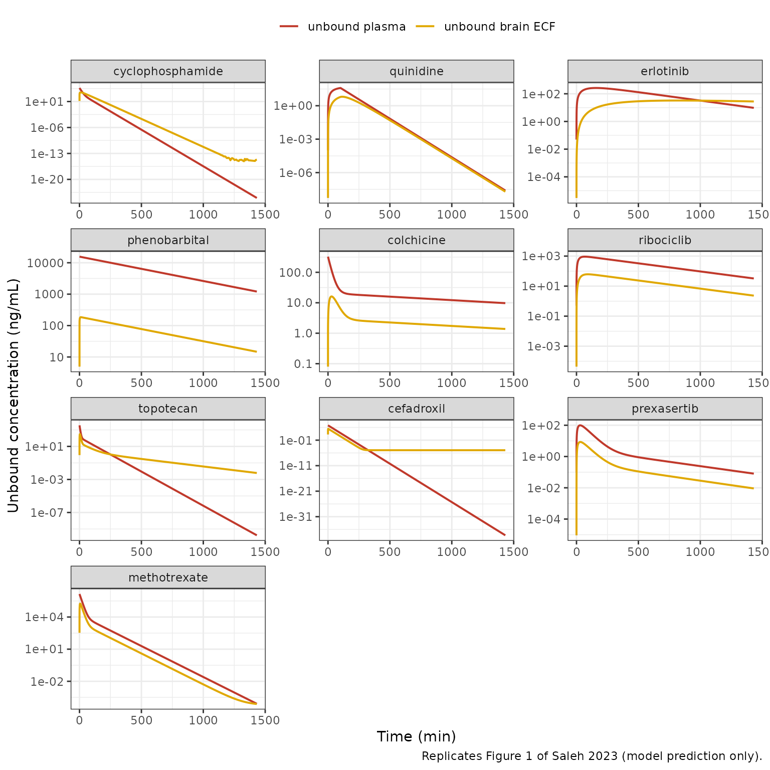
The vertical offset between the two curves within each panel is the
drug’s Kp,uu,BBB, and the lag of the brain-ECF peak behind
the plasma peak is the barrier-limited distribution the model is built
to capture.
Between-subject variability
Table IV reports interindividual variances for a minority of the drugs; for the rest the plasma model is deterministic as published. Ribociclib carries the largest reported variability (variance 0.217 on clearance and 0.676 on absorption), so it is used to show the stochastic layer. The cohort is 200 subjects, the per-arm cap.
The band below is the between-subject prediction interval: it propagates the Table IV interindividual variances through the CNS model. It deliberately excludes residual error, which the paper reports only for the plasma endpoint (brain ECF is a pure prediction with no residual-error term of its own), so the two analytes are shown on the same footing.
set.seed(74)
mod_ribo <- rxode2::rxode2(
  nlmixr2lib::readModelDb("Saleh_2023_ribociclib_mouse_pbpk")
)
#> ℹ parameter labels from comments will be replaced by 'label()'
amt_ribo <- dosing$dose_mgkg[dosing$drug == "ribociclib"] * BW_KG * 1e6
ev_ribo <- rxode2::et(amt = amt_ribo, cmt = "depot")
ev_ribo <- rxode2::et(ev_ribo, seq(0, 1440, length.out = 289))
sim_ribo <- suppressWarnings(
  rxode2::rxSolve(mod_ribo, ev_ribo, nSub = 200, atol = 1e-11, rtol = 1e-9,
                  returnType = "data.frame")
)

vpc_ribo <- sim_ribo |>
  filter(time > 0) |>
  select(sim.id, time, Ccu, Cbrain_ecf) |>
  pivot_longer(c(Ccu, Cbrain_ecf), names_to = "analyte", values_to = "conc") |>
  mutate(analyte = factor(analyte, levels = c("Ccu", "Cbrain_ecf"),
                          labels = c("unbound plasma", "unbound brain ECF"))) |>
  group_by(analyte, time) |>
  summarise(lo = quantile(conc, 0.025), med = median(conc),
            hi = quantile(conc, 0.975), .groups = "drop")

ggplot(vpc_ribo, aes(time, med, colour = analyte, fill = analyte)) +
  geom_ribbon(aes(ymin = lo, ymax = hi), alpha = 0.25, colour = NA) +
  geom_line(linewidth = 0.8) +
  scale_x_continuous("Time (min)") +
  scale_y_log10("Unbound concentration (ng/mL)") +
  scale_colour_manual(values = c("unbound plasma" = "#c0392b",
                                 "unbound brain ECF" = "#e0a800")) +
  scale_fill_manual(values = c("unbound plasma" = "#c0392b",
                               "unbound brain ECF" = "#e0a800")) +
  theme_bw() +
  theme(legend.position = "top") +
  labs(colour = NULL, fill = NULL,
       caption = "Ribociclib 100 mg/kg PO: median and 95% prediction interval, 200 subjects.")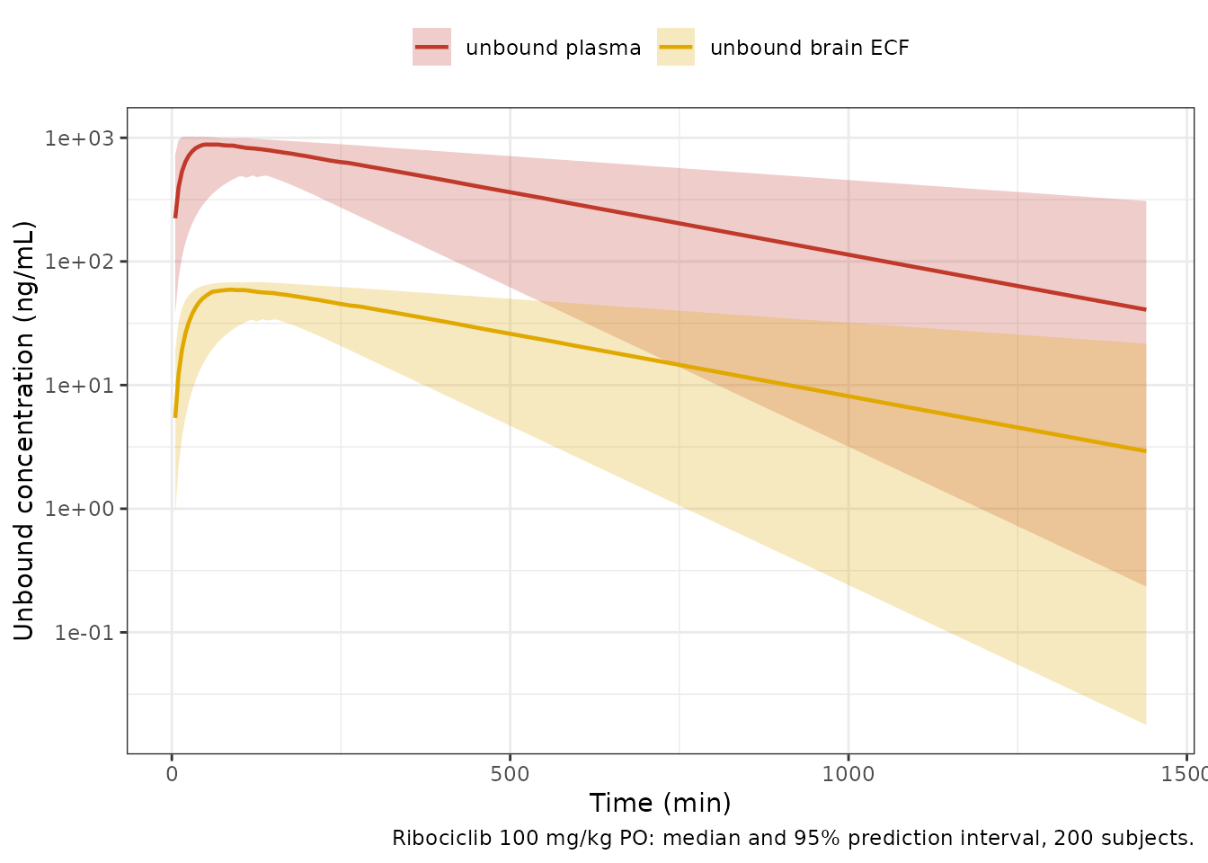
Plasma NCA summary
The paper reports no NCA parameter table, so there is nothing to
compare against numerically here. The plasma NCA below is a descriptive
summary of the ten empirical plasma models the CNS model is driven by,
computed with PKNCA from the same simulations used in Gate
2.
plasma_nca <- nca_res |>
  filter(analyte == "Ccu", PPTESTCD %in% c("cmax", "tmax", "auclast", "half.life")) |>
  select(drug, PPTESTCD, PPORRES) |>
  pivot_wider(names_from = PPTESTCD, values_from = PPORRES) |>
  left_join(dosing, by = "drug") |>
  arrange(match(drug, drugs)) |>
  select(drug, route, dose_mgkg, cmax, tmax, auclast, half.life) |>
  rename("Drug" = drug, "Route" = route, "Dose (mg/kg)" = dose_mgkg,
         "Cmax (ng/mL)" = cmax, "Tmax (min)" = tmax,
         "AUClast (ng*min/mL)" = auclast, "t1/2 (min)" = half.life)

knitr::kable(plasma_nca, digits = c(0, 0, 1, 3, 1, 1, 1),
caption = "Unbound plasma NCA of the ten empirical plasma PK models (descriptive; not a published comparison).")| Drug | Route | Dose (mg/kg) | Cmax (ng/mL) | Tmax (min) | AUClast (ng*min/mL) | t1/2 (min) |
|---|---|---|---|---|---|---|
| cyclophosphamide | IP | 130.0 | 45601.727 | 0.0 | 404306.4 | 21.1 |
| quinidine | IP | 40.0 | 39.192 | 101.2 | 4958.5 | 54.0 |
| erlotinib | PO | 50.0 | 262.038 | 158.1 | 145630.9 | 247.4 |
| phenobarbital | IP | 10.0 | 15625.000 | 0.0 | 8750000.0 | 388.1 |
| colchicine | IV | 1.5 | 326.320 | 0.0 | 46971.3 | 1315.4 |
| ribociclib | PO | 100.0 | 917.962 | 66.9 | 435605.9 | 280.5 |
| topotecan | IV | 4.0 | 3567.182 | 0.0 | 21276.6 | 43.6 |
| cefadroxil | IV | 36.0 | 64285.714 | 0.0 | 927835.1 | 10.0 |
| prexasertib | SC | 10.0 | 98.772 | 29.6 | 10261.2 | 276.1 |
| methotrexate | IV | 1000.0 | 1408794.788 | 0.0 | 18859022.1 | 53.5 |
Assumptions and deviations
Choices that were required because the paper does not state them, and source oddities carried through faithfully.
Assumptions
-
Body weight 0.025 kg. Table IV gives doses in mg/kg
while all volumes are absolute (mL), so a body weight is needed and none
is stated. 0.025 kg is the standard adult laboratory mouse. Corroborated
by Table III note (d), which implies a 0.416 g brain, and by
cefadroxil’s
Vcof 14 mL (0.56 L/kg at 0.025 kg). Every validation gate above is a ratio and so is independent of this value. -
Effective surface areas in Table III are percentages, not
fractions. Table III lists the transcellular / paracellular
effective surface areas under a “(unitless)” header (0.998, 0.006,
0.05). They are percentages. Yamamoto 2017 (reference [43] of that
table) states verbatim that “99.8% of total SA_BBB … is used for
transcellular diffusion, whereas 0.006% of total SA_BBB … [is] used for
paracellular diffusion”, and the authors’ own
physio_para.csvinTingjieGuo/LeiCNS-Sourcestores the rat BBB paracellular value as 6.00E-05. Reading 0.006 as a fraction would inflate paracellular clearance 100-fold. The model files encode this explicitly asfixed(0.006 / 100)so the reading is auditable. -
Per-second to per-minute conversion (x 60) on
DaqandP0. The two published regressions return per-second units while every published table is per-minute. The factor was pinned numerically, not assumed: for rat quinidine the formulas giveP0= 9.60e-4 cm/s -> 0.0576 cm/min against a published 0.058, andDaq= 5.37e-6 cm^2/s -> 3.22e-4 cm^2/min against a published 3.2e-4 (Yamamoto 2017 Table 4). Recomputing Yamamoto Table 5 then givesQt_BBB7.61 vs 7.6,Qp_BBB0.101 vs 0.10,Q_BCM139 vs 140 andQ_LYSO33.4 vs 33. -
CL_wo/CL_oware derived, not printed. LeiCNS-PK3.0 replaced the instantaneous binding factor of LeiCNS-PK1.0 with a mechanistic phospholipid compartment, but no source prints the two clearance magnitudes. Three constraints jointly determine them: the ECF ODE printed in van Valkengoed 2025 Eq 4 showsCL_BC,inacting onPHF_ECF x C_ECFandCL_BC,outonC_BCM; the Saleh 2022 supplement pins the ratioCL_wo / CL_ow = 10^logP; and the LeiCNS convention that a membrane clearance is permeability x surface area is printed as Yamamoto 2017 Eq 8. Applying the same pair to both faces of the membrane is the only assignment that satisfies all three printed steady-state identities simultaneously – which is exactly what Gate 3 tests. It is also numerically immaterial: scaling both by 0.1x and 10x leaves the profiles unchanged, because membrane equilibration is far faster than any observed profile. -
Kp,uuat the two BCSFB barriers is set equal toKp,uu,BBB. Saleh 2023 does not reportKp,uu,LVorKp,uu,CMfor mouse. They are defaulted toKp,uu,BBBfollowing the authors’ owndrug_pk.csvconvention. This cannot affect the brain-ECF endpoint: the CSF chain is strictly downstream ofbrain_ecf, and these values enter theAF_BBBclosed form only through terms inKp,uu,CM x Q_CSF, which with mouseQ_CSF= 3.43e-4 againstQ_CBF= 0.461 mL/min contributes less than 0.1%. -
The empirical plasma model describes TOTAL plasma
concentration.
fu,plasmais listed as a separate parameter of the plasma model in Table IV and is applied to obtain the unbound driving concentration (Ccu <- fu_plasma * Cc). The paper does not state explicitly whether the reported residual error was on the total or the unbound scale. For nine of the ten drugs the residual error is purely proportional, so the distinction is immaterial (a proportional error is invariant to a constant scale factor); it matters only for quinidine’s additive term. -
Residual error and IIV in Table IV are variances.
The table headers say so verbatim (“Interindividual variability (as
variance)”, “Residual unexplained variabilities (as variance)”).
propSdandaddSdare therefore encoded assqrt(<tabulated value>), written out inini()so the published number stays visible. -
Compartment naming. The paper’s
brainMVis encoded as the already-registered canonicalbrain_vascular(cerebral capillary blood, fed at cerebral blood flow) rather than as a new name, and the four CSF subregions use the registeredbrain_csf_lv/brain_csf_tfv/brain_csf_cm/brain_csf_sasfamily. Three genuinely new canonicals were added for this family:brain_icf,brain_cell_membraneandbrain_lysosome.
Source oddities, carried through as published
-
Quinidine’s plasma parameters are
non-physiological. Table IV gives
CL= 46.99 mL/min andVc= 2951.3 mL for a ~25 g mouse – a clearance of roughly 3x mouse cardiac output and a volume of ~118 L/kg. The two are internally consistent and reproduce plausible concentrations for the 101 min zero-order input, so this is almost certainly a flip-flop / identifiability artefact of the in-house fit. Transcribed as published. -
Quinidine is the only drug with a non-zero Duration (101
min), implemented as a zero-order input into the depot which
then empties first-order at
ka= 2.61 min^-1. Dose rows requirerate = -2. -
IP is not always modelled as absorption.
Cyclophosphamide and phenobarbital are intraperitoneal with
ka= 0 and Duration = 0, i.e. modelled as a bolus straight into the central compartment. Faithful to Table IV. -
Cefadroxil has no reported variability at all –
Table IV gives zero for every IIV and both residual variances.
propSdis encoded asfixed(0)rather than invented, so the published plasma model remains an exact deterministic description. - Author spelling slips carried through the paper: “erlotonib” (erlotinib), “cefradroxil” (cefadroxil), “cisterna magma” (cisterna magna), and a “360-ug mouse brain” where 360 uL is meant. The model files use the correct generic names.
- The paper prints no equations. All equations come from the 2021 predecessor and its supplement, as recorded in the source trace above. Nothing was substituted from general PBPK knowledge.
Not extracted
- The paper’s
%AFE/%AAFEprediction-accuracy statistics (Figure 2) are reported per drug but depend on the digitised observed microdialysis data, which are not redistributed here. - The brain-ECF predictions for phenobarbital, prexasertib and methotrexate fall outside two-fold error in the paper’s own assessment (within five-fold). That is a property of the published model, reproduced faithfully rather than tuned away.