Cyclophosphamide (Ahmed 2020)
Source:vignettes/articles/Ahmed_2020_cyclophosphamide.Rmd
Ahmed_2020_cyclophosphamide.RmdModel and source
- Citation: Ahmed JH, Makonnen E, Bisaso RK, Mukonzo JK, Fotoohi A, Aseffa A, Howe R, Hassan M, Aklillu E. Population Pharmacokinetic, Pharmacogenetic, and Pharmacodynamic Analysis of Cyclophosphamide in Ethiopian Breast Cancer Patients. Front Pharmacol. 2020;11:406. doi:10.3389/fphar.2020.00406
- Description: One-compartment population PK model for intravenous cyclophosphamide in Ethiopian women with breast cancer (Ahmed 2020), with the cyclophosphamide dosage regimen (500 vs 600 mg/m^2 based) on clearance and volume and body surface area on volume, linked to a linear direct-response (empiric) model of absolute neutrophil count driven by the cumulative cyclophosphamide AUC.
- Article: https://doi.org/10.3389/fphar.2020.00406 (open access)
A literature check on 2026-09-26 (Europe PMC) found no erratum or correction for this article. The article’s supplementary files are the figure images only; there is no NONMEM control stream.
Population
Ahmed 2020 enrolled 267 women with breast cancer at the radiotherapy centre of Tikur Anbessa Specialized Hospital, Addis Ababa, Ethiopia, who were starting their first cycle of cyclophosphamide-containing chemotherapy. Median age was 38 years (IQR 33-48), mean body surface area (BSA) 1.59 +/- 0.20 m^2 and mean body mass index 23.78 +/- 4.8 kg/m^2 (Table 1). Patients received cyclophosphamide as a 30-min IV infusion either at 600 mg/m^2 (AC or AC-T regimens; 161 patients, 60.3%) or at 500 mg/m^2 (FAC regimen, which adds 5-fluorouracil; 106 patients, 39.7%). The median absolute dose was 930 mg (650-1,150 mg) in the 600 mg/m^2 group and 777.5 mg (600-1,000 mg) in the 500 mg/m^2 group. The analysis used 532 plasma concentrations (about two per patient, mostly at 1-6 h after the start of infusion; 17 patients were sampled up to 22 h) and absolute neutrophil counts (ANC) at baseline and on day 20. Median baseline ANC was 3645.5 cells/mm^3 (Table 1; the table header says 10^3 cells/mm^3 but the values are cells/mm^3).
The same information is available programmatically via
readModelDb("Ahmed_2020_cyclophosphamide")()$population.
Source trace
| Equation / parameter | Value | Source location |
|---|---|---|
| Structure: one compartment, IV infusion, first-order elimination | – | Results ‘Population Pharmacokinetic Modeling’ |
lcl (CL, 600 mg/m^2 regimen) |
5.41 L/h | Table 3, final model |
lvc (VD, 600 mg/m^2 regimen, BSA 1.58 m^2) |
46.5 L | Table 3, final model |
e_dose_high_cl (500 mg/m^2 regimen on CL,
1 + THETA) |
-0.323 | Table 4 |
e_dose_high_vc (500 mg/m^2 regimen on VD,
1 + THETA) |
-0.371 | Table 4 |
e_bsa_vc ((BSA/1.58)^THETA on VD) |
0.861 | Table 4; Methods Equation 1 |
etalcl |
46.4% CV -> 0.19500 | Table 3, final model; %CV = sqrt(exp(omega^2) - 1)
(Methods) |
etalvc |
35.9% CV -> 0.12123 | Table 3, final model |
addSd |
1.54 mg/L | Table 3, ‘Additive error 1’ |
PD structure: ANC = ANC0 + slope * AUC
|
– | Methods Equation 5; Results ‘Pharmacodynamic Modeling’; Figure 7 |
lrbase_anc (ANC0) |
3450 cells/mm^3 | Results ‘Pharmacodynamic Modeling’ |
slope_anc |
-1.42 (cells/mm^3)/(umol*h/L) | Results ‘Pharmacodynamic Modeling’ |
propSd_ANC, addSd_ANC
|
0 (fixed) | Combined error selected, magnitudes not reported |
| AUC unit conversion, MW 261.09 g/mol | – | Table 3 reports AUC in umol*h/L; molecular weight of anhydrous cyclophosphamide |
Virtual cohort
Two arms of 200 patients each, one per regimen. BSA is drawn from a normal distribution with the Table 1 mean and SD, truncated to 1.2-2.2 m^2; the absolute dose is the regimen dose per m^2 times the patient’s BSA, infused over 30 min.
set.seed(20200423)
rxode2::rxSetSeed(20200423)
n_per_arm <- 200

cohort <- tibble::tibble(
  id = seq_len(2 * n_per_arm),
  arm = rep(c("500 mg/m^2", "600 mg/m^2"), each = n_per_arm),
  DOSE_HIGH = rep(c(0L, 1L), each = n_per_arm),
  BSA = pmin(pmax(rnorm(2 * n_per_arm, 1.59, 0.20), 1.2), 2.2)
) |>
  dplyr::mutate(dose = ifelse(DOSE_HIGH == 1L, 600, 500) * BSA)

obs_times <- c(0, 0.25, 0.5, 0.75, 1, 1.5, 2, 3, 4, 5, 6, 8, 10, 12, 16, 22, 24, 36, 48, 480)

make_events <- function(cohort, obs_times) {
  doses <- cohort |>
    dplyr::transmute(
      id, time = 0, amt = dose, rate = dose / 0.5, evid = 1L,
      cmt = "central", dvid = NA_integer_, DOSE_HIGH, BSA
    )
  obs <- tidyr::expand_grid(id = cohort$id, time = obs_times) |>
    dplyr::left_join(cohort |> dplyr::select(id, DOSE_HIGH, BSA), by = "id") |>
    dplyr::mutate(
      amt = NA_real_, rate = NA_real_, evid = 0L,
      cmt = NA_character_, dvid = 1L
    )
  dplyr::bind_rows(doses, obs) |>
    dplyr::arrange(id, time, dplyr::desc(evid)) |>
    as.data.frame()
}

events <- make_events(cohort, obs_times)
Simulation
mod <- readModelDb("Ahmed_2020_cyclophosphamide")

sim <- rxode2::rxSolve(
  mod, events,
  keep = c("DOSE_HIGH", "BSA"),
  returnType = "data.frame", useLinCmt = FALSE
) |>
  dplyr::left_join(cohort |> dplyr::select(id, arm), by = "id")
#> ℹ parameter labels from comments will be replaced by 'label()'

# Typical-value solve (no between-subject variability, no residual error)
sim_tv <- rxode2::rxSolve(
  mod, events,
  keep = c("DOSE_HIGH", "BSA"),
  returnType = "data.frame", useLinCmt = FALSE,
  omega = NA, sigma = NA
) |>
  dplyr::left_join(cohort |> dplyr::select(id, arm), by = "id")
Typical-value check against the closed form
A one-compartment infusion model has an analytic solution. At the end
of a 0.5 h infusion of dose D the concentration is
D / (0.5 * CL) * (1 - exp(-k * 0.5)) with
k = CL / V, and the day-20 AUC is D / CL. Both
sides use the same parameters, so the difference is numerical error only
and a tight bound is appropriate.
tv_par <- cohort |>
  dplyr::mutate(
    cl = 5.41 * (1 - 0.323 * (1 - DOSE_HIGH)),
    vc = 46.5 * (BSA / 1.58)^0.861 * (1 - 0.371 * (1 - DOSE_HIGH)),
    k = cl / vc,
    c_eoi = dose / (0.5 * cl) * (1 - exp(-k * 0.5)),
    auc_umol = dose / cl * 1000 / 261.09,
    anc_d20 = 3450 - 1.42 * auc_umol
  )

chk <- sim_tv |>
  dplyr::filter(time %in% c(0.5, 480)) |>
  dplyr::select(id, time, Cc, ANC) |>
  tidyr::pivot_wider(names_from = time, values_from = c(Cc, ANC)) |>
  dplyr::left_join(tv_par, by = "id")

stopifnot(
  all(abs(chk$Cc_0.5 / chk$c_eoi - 1) < 1e-4),
  all(abs(chk$ANC_480 - chk$anc_d20) < 0.5),
  all(abs(sim_tv$ANC[sim_tv$time == 0] - 3450) < 1e-8)
)

tv_par |>
  dplyr::group_by(arm) |>
  dplyr::summarise(
    `CL (L/h)` = signif(unique(cl), 3),
    `median V (L)` = signif(median(vc), 3),
    `median t1/2 (h)` = signif(median(log(2) / k), 3),
    .groups = "drop"
  ) |>
  dplyr::rename(Regimen = arm) |>
knitr::kable(caption = "Typical-value PK parameters by regimen in the virtual cohort.")| Regimen | CL (L/h) | median V (L) | median t1/2 (h) |
|---|---|---|---|
| 500 mg/m^2 | 3.66 | 30.1 | 5.70 |
| 600 mg/m^2 | 5.41 | 46.3 | 5.93 |
Replicate published figures
The paper has no concentration-time profile figure beyond the pcVPC of Figure 3, whose axes are prediction corrected. The panel below shows the simulated 5th, 50th and 95th percentiles over the sampling window used in the study (up to 22 h after the start of infusion).
sim |>
  dplyr::filter(time <= 24) |>
  dplyr::group_by(arm, time) |>
  dplyr::summarise(
    lo = quantile(Cc, 0.05), med = median(Cc), hi = quantile(Cc, 0.95),
    .groups = "drop"
  ) |>
  ggplot(aes(time, med, colour = arm, fill = arm)) +
  geom_ribbon(aes(ymin = lo, ymax = hi), alpha = 0.2, colour = NA) +
  geom_line() +
  scale_y_log10() +
  labs(x = "Time after start of infusion (h)", y = "Cyclophosphamide (mg/L)",
       colour = "Regimen", fill = "Regimen")
#> Warning in scale_y_log10(): log-10 transformation introduced infinite values.
#> log-10 transformation introduced infinite values.
#> log-10 transformation introduced infinite values.
#> log-10 transformation introduced infinite values.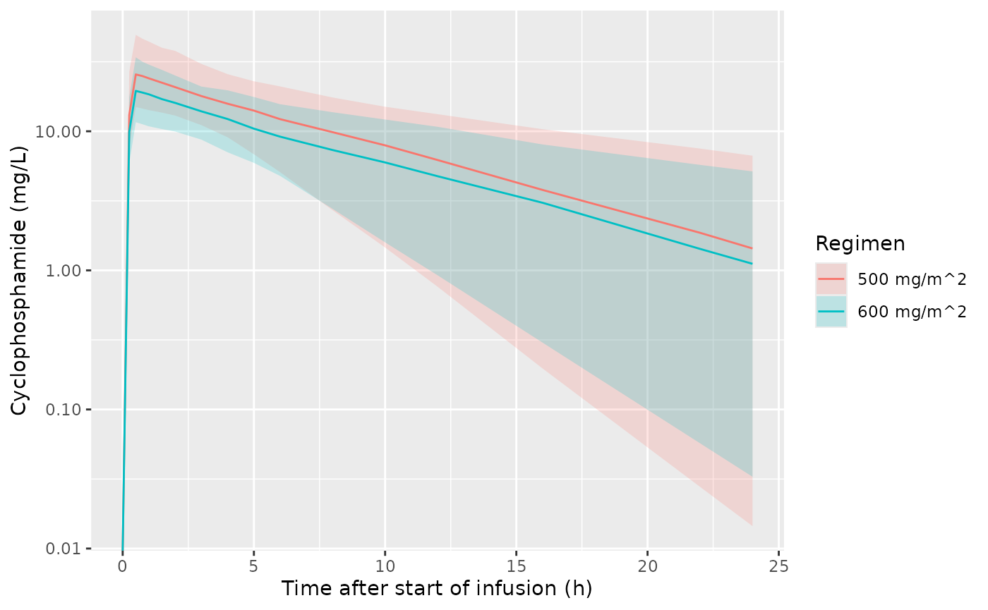
Simulated cyclophosphamide concentrations (median and 90% interval) over the Ahmed 2020 sampling window, by regimen; compare the range of Figure 3 of Ahmed 2020.
anc_d20 <- sim |>
  dplyr::filter(time == 480) |>
  dplyr::mutate(auc_umol = auc * 1000 / 261.09)

ggplot(anc_d20, aes(auc_umol, ANC, colour = arm)) +
  geom_point(alpha = 0.5) +
  geom_hline(yintercept = 3450, linetype = 2) +
  labs(x = "Cyclophosphamide AUC0-day20 (umol*h/L)",
       y = "Predicted ANC on day 20 (cells/mm^3)", colour = "Regimen")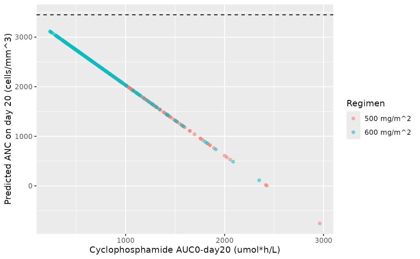
Model-predicted day-20 ANC against the cyclophosphamide AUC; replicates the range of the population predictions in Figure 7 of Ahmed 2020 (baseline predictions at 3450 cells/mm^3, day-20 predictions mostly between about 2000 and 3100 cells/mm^3).
PKNCA validation
Concentrations are converted to umol/L so that the AUC is on the
umol*h/L scale Ahmed 2020 Table 3 uses. The paper’s derived PK summaries
(Table 3) are for the whole cohort, so the NCA is also run on the pooled
cohort, grouped as All, next to the per-regimen
results.
# Late samples (36 h onward) sit at the solver's numerical noise floor and can
# be negative by ~1e-30; PKNCA returns NaN for AUClast on any profile with a
# negative concentration, so those are floored at zero.
conc_df <- sim |>
  dplyr::filter(!is.na(Cc)) |>
  dplyr::mutate(conc_umol = pmax(Cc, 0) * 1000 / 261.09) |>
  dplyr::select(id, time, conc_umol, arm)

dose_df <- cohort |>
  dplyr::transmute(id, time = 0, amt = dose, arm)

run_nca <- function(conc_df, dose_df) {
  conc_obj <- PKNCA::PKNCAconc(conc_df, conc_umol ~ time | arm + id)
  dose_obj <- PKNCA::PKNCAdose(dose_df, amt ~ time | arm + id,
                               route = "intravascular", duration = 0.5)
  intervals <- data.frame(
    start = 0, end = 480,
    cmax = TRUE, tmax = TRUE, auclast = TRUE, half.life = TRUE
  )
  PKNCA::pk.nca(PKNCA::PKNCAdata(conc_obj, dose_obj, intervals = intervals))
}

nca_arm <- run_nca(conc_df, dose_df)
nca_all <- run_nca(conc_df |> dplyr::mutate(arm = "All"),
                   dose_df |> dplyr::mutate(arm = "All"))

summary(nca_arm)
#>  start end        arm   N    auclast        cmax                 tmax
#>      0 480 500 mg/m^2 200 845 [49.0]  100 [38.6] 0.500 [0.500, 0.500]
#>      0 480 600 mg/m^2 200 640 [48.7] 74.5 [33.9] 0.500 [0.500, 0.500]
#>    half.life
#>  6.74 [4.08]
#>  6.80 [4.69]
#>
#> Caption: auclast, cmax: geometric mean and geometric coefficient of variation; tmax: median and range; half.life: arithmetic mean and standard deviation; N: number of subjects
summary(nca_all)
#>  start end arm   N    auclast        cmax                 tmax   half.life
#>      0 480 All 400 736 [51.2] 86.3 [39.5] 0.500 [0.500, 0.500] 6.77 [4.39]
#>
#> Caption: auclast, cmax: geometric mean and geometric coefficient of variation; tmax: median and range; half.life: arithmetic mean and standard deviation; N: number of subjects
Comparison against published values
Ahmed 2020 Table 3 reports the median of the empirical Bayes AUC0-day20 (565.7 umol*h/L) and half-life (5.48 h) for the whole cohort.
published <- tibble::tribble(
  ~arm, ~auclast, ~half.life,
  "All", 565.7, 5.48
)

cmp <- nlmixr2lib::ncaComparisonTable(
  simulated = nca_all,
  reference = published,
  by = "arm",
  units = c(auclast = "umol*h/L", half.life = "h"),
  tolerance_pct = 20
)
knitr::kable(cmp, caption = "Simulated vs. published (Ahmed 2020 Table 3). * differs from reference by >20%.")| NCA parameter | arm | Reference | Simulated | % diff |
|---|---|---|---|---|
| AUClast (umol*h/L) | All | 566 | 738 | +30.5%* |
| t½ (h) | All | 5.48 | 5.62 | +2.6% |
The simulated median half-life agrees with Table 3. The simulated
median AUC is about 30% higher than the 565.7 umolh/L of Table 3.
AUC0-day20 is dose / CL independent of the volume, and the
typical-value AUC alone is about 660 umolh/L in the 600 mg/m^2 arm
(930 mg / 5.41 L/h) and about 810 umol*h/L in the 500 mg/m^2 arm, so the
gap is a property of the published parameter set and not of the
simulation. Table 3 does not state how its derived AUC was computed; it
was not used to adjust any parameter.
The regimen-specific clearances reported in the Results (mean 3.97 L/h for the 500 mg/m^2 regimen and 5.81 L/h for the 600 mg/m^2 regimen) and the 600 mg/m^2-regimen half-lives by BSA group (4.78 h below 1.5 m^2, 5.42 h for 1.5-1.74 m^2, 6.71 h above 1.75 m^2) are empirical Bayes summaries; the simulated equivalents are shown below. With about two samples per patient the empirical Bayes estimates are shrunk towards the typical value, so the simulated spread across BSA groups is expected to be at least as wide as the published one; the published half-lives are not stated as means or medians.
ind <- sim |>
  dplyr::filter(time == 0.5) |>
  dplyr::select(id, arm, BSA, cl, vc, kel)

ind |>
  dplyr::group_by(arm) |>
  dplyr::summarise(`mean CL (L/h)` = signif(mean(cl), 3), .groups = "drop") |>
  dplyr::mutate(`published mean CL (L/h)` = c(3.97, 5.81)) |>
  dplyr::rename(Regimen = arm) |>
knitr::kable(caption = "Mean individual clearance by regimen (Ahmed 2020 Results).")| Regimen | mean CL (L/h) | published mean CL (L/h) |
|---|---|---|
| 500 mg/m^2 | 4.07 | 3.97 |
| 600 mg/m^2 | 6.21 | 5.81 |
ind |>
  dplyr::filter(arm == "600 mg/m^2") |>
  dplyr::mutate(bsa_group = cut(BSA, c(0, 1.5, 1.75, Inf),
                                labels = c("< 1.5", "1.5-1.74", ">= 1.75"),
                                right = FALSE)) |>
  dplyr::group_by(bsa_group) |>
  dplyr::summarise(`simulated median t1/2 (h)` = signif(median(log(2) / kel), 3),
                   .groups = "drop") |>
  dplyr::mutate(`published t1/2 (h)` = c(4.78, 5.42, 6.71)) |>
  dplyr::rename(`BSA group (m^2)` = bsa_group) |>
knitr::kable(caption = "Half-life by BSA group in the 600 mg/m^2 regimen (Ahmed 2020 Results).")| BSA group (m^2) | simulated median t1/2 (h) | published t1/2 (h) |
|---|---|---|
| < 1.5 | 5.27 | 4.78 |
| 1.5-1.74 | 5.87 | 5.42 |
| >= 1.75 | 6.56 | 6.71 |
Assumptions and deviations
-
Sign of the PD slope. Equation 5 is printed as
Y = ANCo - slope * AUCand the Results giveslope = -1.42. Taken literally the count would rise with exposure, which contradicts the Results (“a one unit increase in the AUC of CPA was associated with a decrease in the neutrophil count by 1.42”), the Discussion, and Figure 7, where every population prediction lies at or below- The model therefore uses
ANC = ANC0 + slope * AUCwith the reportedslope = -1.42.
- The model therefore uses
- AUC unit in the PD model. The paper does not state the AUC unit in the PD fit. Table 3 reports AUC0-day20 in umolh/L, and only that unit reproduces the Figure 7 population predictions (about 2000-3100 cells/mm^3 on day 20 for an interquartile AUC of 445-828 umolh/L). The concentration state is in mg/L, so the AUC is converted with the cyclophosphamide molecular weight 261.09 g/mol, which the paper does not print.
- AUC regressor over time. The model regresses the ANC on the running AUC integral, so it returns ANC0 at baseline and the Equation 5 value on day 20 (by which time the AUC is complete). The paper only fitted those two time points; predictions at intermediate times have no source support.
- PD residual error and variability. A combined proportional and additive residual error was selected for ANC but its magnitudes are not reported, so both are fixed to 0. No between-subject variability on ANC0 or the slope is reported; Figure 7 shows individual and population predictions that coincide, consistent with none being estimated.
- Second additive PK residual. Table 3 lists a second additive error of 0.0001 mg/mL (0.1 mg/L) whose role is not described. It is not encoded; added in quadrature to 1.54 mg/L it would change the residual SD by 0.2%.
- Residual magnitude as an SD. The 1.54 mg/L is taken as a standard deviation because it is reported in concentration units.
- BSA reference. Methods Equation 1 describes the BSA normalising value as the median; Table 4 prints 1.58 m^2, which is used.
-
Regimen covariate. The 500 mg/m^2 (FAC) and 600
mg/m^2 (AC, AC-T) regimens differ in co-administered drugs as well as in
cyclophosphamide dose, so the covariate is a regimen effect. It is
carried in the
DOSE_HIGHcolumn (1 = 600 mg/m^2), with the Table 4 coefficient applied to the 500 mg/m^2 complement. -
Genotype effects. CYP3A5 and CYP2C9 genotype
associations are post hoc analyses of empirical Bayes estimates and are
not part of the NONMEM model; they are documented in
covariatesDataExcluded. - Virtual cohort. BSA is drawn from a truncated normal with the Table 1 mean and SD; the paper gives no BSA distribution by regimen.