Febuxostat (Iwama 2024)
Source:vignettes/articles/Iwama_2024_febuxostat.Rmd
Iwama_2024_febuxostat.RmdModel and source
- Citation: Iwama R, Nishida K, Ishii D, Iijima T. An integrated population pharmacokinetic model of febuxostat in pediatric patients with hyperuricemia including gout and adult population of healthy subjects and patients with renal dysfunction. Pharmacol Res Perspect. 2024;12(6):e70032. doi:10.1002/prp2.70032.
- Description: Integrated two-compartment population PK model for febuxostat spanning Japanese pediatric patients with hyperuricemia including gout and a Japanese adult population of healthy subjects and patients with renal dysfunction (Iwama 2024). First-order absorption from a depot with an absorption lag time, first-order elimination, and apparent (oral) disposition parameters. Apparent clearance is a power function of body weight and of BSA-normalized estimated glomerular filtration rate, each centered on the pooled-analysis median (60.6 kg, 98.6 mL/min/1.73 m^2). Relative bioavailability is reduced to 0.838 when the dose is taken fed, with the fasted state as the structural anchor. Age was screened but not retained, which is what makes the single model applicable across the pediatric and adult populations.
- Article: https://doi.org/10.1002/prp2.70032
Febuxostat is a xanthine oxidoreductase inhibitor used for urate-lowering therapy. Iwama and colleagues pooled six Japanese studies to build a single integrated population PK model that spans pediatric patients with hyperuricemia including gout and an adult population of healthy subjects and patients with renal dysfunction. The purpose of the integration was regulatory: to justify half the adult dose for pediatric patients weighing < 40 kg and the full adult dose for those weighing >= 40 kg, and to confirm that no dose adjustment is needed for mild-to-moderate renal impairment.
The structural model is a two-compartment disposition model with first-order absorption from a depot, an absorption lag time, and first-order elimination. All disposition parameters are apparent (oral) quantities because no intravenous data were available. Apparent clearance carries power-function effects of body weight and of BSA-normalized estimated glomerular filtration rate (eGFR), each centered on the pooled-analysis median. Relative bioavailability is reduced when the dose is taken fed.
The single most consequential result of the paper is a negative one: age was not retained as a covariate. That is what makes one model applicable to both the pediatric and the adult population, and it is the basis of the paper’s weight-band dosing recommendation.
Population
The analysis pooled 2611 plasma febuxostat concentration records from 142 Japanese subjects across six studies (Table 1 of the source):
- 29 pediatric patients aged 8 to 18 years with hyperuricemia including gout, from two Phase 2 studies (evaluation phase and continuation phase). 10 weighed < 40 kg and 19 weighed >= 40 kg. Dosing was weight-banded: 5, 10, 20 or 30 mg once daily for the < 40 kg band and 10, 20, 40 or 60 mg once daily for the >= 40 kg band, given for 52 weeks with up-titration as needed. 110 records came from the < 40 kg band and 190 from the >= 40 kg band.
- 113 adult subjects, comprising 92 healthy Japanese adult males from three Phase 1 studies (10-160 mg, single or repeated, fasted or fed) and 21 adults from a Phase 1 repeated-dose study of 20 mg in subjects with normal renal function or renal dysfunction. 2311 records.
The cohort spans 26.7 to 94.3 kg in body weight and 20.9 to 145.3 mL/min/1.73 m^2 in eGFR, covering normal renal function through severe renal dysfunction (87 normal, 34 mild, 19 moderate, 2 severe across the whole analysis set). The cohort is overwhelmingly male (133 of 142; only 6 pediatric and 3 adult females), which is why sex was not screened as a covariate. The pediatric patients had a higher prevalence of reduced renal function than the adults, which is the clinical situation the paper set out to address.
The pooled-analysis medians used for covariate centering are 60.6 kg and 98.6 mL/min/1.73 m^2. Note that these are medians of the pooled data set and so match neither the pediatric (46.70 kg) nor the adult (61.30 kg) median in Table 1.
The same information is available programmatically via the model’s
population metadata:
str(rxode2::rxode(readModelDb("Iwama_2024_febuxostat"))$population)
#> ℹ parameter labels from comments will be replaced by 'label()'
#> List of 15
#>  $ species       : chr "human"
#>  $ n_subjects    : num 142
#>  $ n_studies     : num 6
#>  $ age_range     : chr "8-72 years (pediatric 8-18; adult 20-72)"
#>  $ age_median    : chr "13.0 years (pediatric); 24.0 years (adult)"
#>  $ weight_range  : chr "26.7-94.3 kg"
#>  $ weight_median : chr "46.70 kg (pediatric); 61.30 kg (adult); 60.6 kg (pooled analysis median used for covariate centering)"
#>  $ sex_female_pct: num 6.3
#>  $ race_ethnicity: Named num 100
#>   ..- attr(*, "names")= chr "Japanese"
#>  $ disease_state : chr "29 pediatric patients with hyperuricemia including gout; 113 adults who were healthy or had renal dysfunction. "| __truncated__
#>  $ dose_range    : chr "Pediatric: 5, 10, 20 or 30 mg once daily orally for body weight < 40 kg and 10, 20, 40 or 60 mg once daily for "| __truncated__
#>  $ regions       : chr "Japan"
#>  $ n_observations: num 2611
#>  $ renal_function: chr "Deliberately enriched for renal impairment. Pediatric eGFR median 76.65 (range 33.9-145.3) mL/min/1.73 m^2; adu"| __truncated__
#>  $ notes         : chr "Pooled analysis of six Japanese studies: two Phase 2 pediatric studies (Study 1 evaluation phase, Study 2 conti"| __truncated__
Source trace
The per-parameter origin is recorded as an in-file comment next to
each ini() entry in
inst/modeldb/specificDrugs/Iwama_2024_febuxostat.R. The
table below collects them in one place for review.
| Equation / parameter | Value | Source location |
|---|---|---|
lcl (CL/F) |
6.53 L/h | Table 2 row CL/F; restated in Section 3.3 and as the
intercept of the Section 3.3 CL/F equation |
lvc (V2/F) |
19.4 L | Table 2 row V2/F; Section 3.3 |
lq (Q/F) |
1.80 L/h | Table 2 row Q/F; Section 3.3 |
lvp (V3/F) |
15.6 L | Table 2 row V3/F; Section 3.3 |
lka (Ka) |
3.43 1/h | Table 2 row Ka; Section 3.3 |
ltlag (ALAG1) |
0.437 h | Table 2 row ALAG1; Section 3.3 |
lfdepot (F fasted) |
1 (fixed) | Section 3.3 F (FASTED) = 1; no typical-value row in
Table 2 |
e_wt_cl (CLWGT) |
0.584 | Table 2 row CLWGT; Section 3.3 CL/F equation exponent
on WGT/60.6
|
e_crcl_cl (CLEGFR) |
0.324 | Table 2 row CLEGFR; Section 3.3 CL/F equation exponent
on EGFR/98.6
|
e_fed_fdepot (F1 FED) |
0.838 | Table 2 row F1 (FED); Section 3.3
F1 (FED) = 0.838
|
| CL/F covariate equation | 6.53 * (WGT/60.6)^0.584 * (EGFR/98.6)^0.324 |
Section 3.3, displayed equation |
| Weight centering value | 60.6 kg | Section 3.3 equation; Section 3.5 “median body weight (60.6 kg)” |
| eGFR centering value | 98.6 mL/min/1.73 m^2 | Section 3.3 equation; Section 3.5; Figure 3 and Figure 5 captions |
etalcl + etalvc block |
0.0662 / 0.0483 / 0.0638 | Table 2 rows omega CL/F^2,
omega CL/F-V2/F^2, omega V2/F^2; block stated
in Section 3.3 |
etalq + etalvp block |
0.411 / 0.307 / 0.259 | Table 2 rows omega Q/F^2,
omega Q/F-V3/F^2, omega V3/F^2; block stated
in Section 3.3 |
etalka |
2.34 | Table 2 row omega Ka^2
|
| IIV on ALAG1 and on F | 0 (fixed) | Table 2 rows omega ALAG1^2 and
omega F1 (FED)^2, both reported as 0, FIX
|
expSd |
sqrt(0.136) = 0.369 |
Table 2 row sigma^2 (exponential error); error model
named in Section 3.3 |
| Two-compartment structure with first-order absorption and lag | n/a | Section 3.3 and Discussion paragraph 1 |
| Absence of an age effect | n/a | Section 3.3 “Age was not included as a significant covariate”; Section 3.7 |
Variance scale
Every variance term above is a variance, not a standard deviation. The Table 2 footnote states the conversions used by the authors, and both are reproduced exactly by the encoded values, which pins the scale beyond doubt:
omega2 <- c("CL/F" = 0.0662, "V2/F" = 0.0638, "Q/F" = 0.411,
            "V3/F" = 0.259, "Ka" = 2.34)
tibble::tibble(
  Parameter          = names(omega2),
  `omega^2 (Table 2)` = unname(omega2),
  `CV% recomputed`   = round(100 * sqrt(exp(unname(omega2)) - 1), 1),
  `CV% printed`      = c(26.2, 25.7, 71.3, 54.4, 306.3)
) |>
  knitr::kable(
    caption = paste(
      "Between-subject variability scale check. Table 2 footnote:",
      "CV(%) = SQRT(EXP(omega^2) - 1) x 100."
    )
)| Parameter | omega^2 (Table 2) | CV% recomputed | CV% printed |
|---|---|---|---|
| CL/F | 0.0662 | 26.2 | 26.2 |
| V2/F | 0.0638 | 25.7 | 25.7 |
| Q/F | 0.4110 | 71.3 | 71.3 |
| V3/F | 0.2590 | 54.4 | 54.4 |
| Ka | 2.3400 | 306.3 | 306.3 |
The residual term follows the other footnote convention,
CV(%) = sigma x 100: sqrt(0.136) = 0.3688,
i.e. 36.9%, matching the printed value. NONMEM’s exponential residual
Y = F * EXP(EPS(1)) is nlmixr2’s lnorm()
residual, whose argument is the log-scale standard deviation, so
expSd = sqrt(0.136).
The two correlation blocks reported in Section 3.3 imply correlations of 0.743 (CL/F with V2/F) and 0.941 (Q/F with V3/F). Both are strictly inside the unit interval, so both blocks are positive definite as published and no numerical nudging was required.
Covariate model verification
Before simulating anything, the encoded covariate equation is checked directly against the numbers the paper prints in its own sensitivity analysis (Section 3.5, plotted as Figure 3). This is the strictest available test of the encoding, because those percentages are closed-form consequences of the CL/F equation and are stated to three significant figures.
The clearances below are read out of the solved model rather than recomputed by hand, so this checks the model file as written, not a transcription of it.
mod_typical <- rxode2::zeroRe(readModelDb("Iwama_2024_febuxostat"))
#> ℹ parameter labels from comments will be replaced by 'label()'

sens_cov <- tibble::tribble(
  ~scenario,                              ~WT,   ~CRCL,
  "Reference (WT 60.6 kg, eGFR 98.6)",    60.6,   98.6,
  "Body weight 82.6 kg (95th pctile)",    82.6,   98.6,
  "Body weight 38.4 kg (5th pctile)",     38.4,   98.6,
  "eGFR 60 (mild dysfunction)",           60.6,   60.0,
  "eGFR 30 (moderate dysfunction)",       60.6,   30.0,
  "eGFR 15 (severe dysfunction)",         60.6,   15.0
) |>
  mutate(id = row_number(), FED = 0)

sens_ev <- bind_rows(
  sens_cov |> mutate(time = 0, amt = 20, evid = 1L, cmt = "depot"),
  sens_cov |> mutate(time = 1, amt = NA_real_, evid = 0L, cmt = "central")
) |>
  arrange(id, time, desc(evid)) |>
  as.data.frame()

sens_sim <- rxode2::rxSolve(
  mod_typical, events = sens_ev, keep = c("scenario", "WT", "CRCL")
) |>
  as.data.frame() |>
  filter(!is.na(Cc)) |>
  group_by(scenario) |>
  summarise(cl = first(cl), .groups = "drop")
#> ℹ omega/sigma items treated as zero: 'etalcl', 'etalvc', 'etalq', 'etalvp', 'etalka'
#> Warning: multi-subject simulation without without 'omega'

cl_ref <- sens_sim$cl[sens_sim$scenario == "Reference (WT 60.6 kg, eGFR 98.6)"]

sens_tbl <- sens_sim |>
  mutate(
    `CL/F (L/h)`        = round(cl, 3),
    `Relative to ref %` = round(100 * cl / cl_ref, 1)
  ) |>
  left_join(
    tibble::tibble(
      scenario = c("Reference (WT 60.6 kg, eGFR 98.6)",
                   "Body weight 82.6 kg (95th pctile)",
                   "Body weight 38.4 kg (5th pctile)",
                   "eGFR 60 (mild dysfunction)",
                   "eGFR 30 (moderate dysfunction)",
                   "eGFR 15 (severe dysfunction)"),
      `Published %` = c(100.0, 119.8, 76.6, 100 - 14.9, 100 - 27.5, 100 - 45.7)
    ),
    by = "scenario"
  ) |>
  select(Scenario = scenario, `CL/F (L/h)`, `Relative to ref %`, `Published %`)

knitr::kable(
  sens_tbl,
  caption = paste(
    "Covariate sensitivity check against Iwama 2024 Section 3.5 / Figure 3.",
    "Published values are read from the Section 3.5 prose."
  )
)| Scenario | CL/F (L/h) | Relative to ref % | Published % |
|---|---|---|---|
| Body weight 38.4 kg (5th pctile) | 5.003 | 76.6 | 76.6 |
| Body weight 82.6 kg (95th pctile) | 7.825 | 119.8 | 119.8 |
| Reference (WT 60.6 kg, eGFR 98.6) | 6.530 | 100.0 | 100.0 |
| eGFR 15 (severe dysfunction) | 3.548 | 54.3 | 54.3 |
| eGFR 30 (moderate dysfunction) | 4.441 | 68.0 | 72.5 |
| eGFR 60 (mild dysfunction) | 5.559 | 85.1 | 85.1 |
Five of the six rows reproduce the published figure exactly, to every printed digit: 119.8% and 76.6% for the body-weight extremes, and 14.9% and 45.7% reductions for eGFR 60 and eGFR 15. The reference row is 100% by construction.
The eGFR 30 row does not agree, and the disagreement
is a defect in the paper rather than in the encoding. The paper’s own
CL/F equation gives (30/98.6)^0.324 = 0.680, i.e. a 32.0%
reduction, whereas Section 3.5 prints 27.5%. The two bracketing points
on the same curve, computed with the same exponent, match the published
values exactly, so the exponent and the centering value are certainly
right and the isolated 27.5% is an internal inconsistency in the paper’s
prose. Per the standing convention of trusting a printed equation over
conflicting prose, the equation is what is encoded. This is recorded
again under Assumptions and deviations below.
The food effect provides one further closed-form check. The
Discussion states that “relative bioavailability, AUCtau,ss, and Cmax,ss
were each reduced by 16.2% in the fed group”, and 1 - 0.838
= 0.162 exactly.
The model’s terminal half-life at the reference covariate values can also be compared against the observed post hoc estimates:
k10 <- 6.53 / 19.4; k12 <- 1.80 / 19.4; k21 <- 1.80 / 15.6
s   <- k10 + k12 + k21
beta <- 0.5 * (s - sqrt(s^2 - 4 * k21 * k10))
cat(sprintf(
  "Closed-form terminal half-life at reference covariates: %.2f h\n%s\n",
  log(2) / beta,
  "Published adult post hoc t1/2 (Table 3): 7.98 +/- 0.97 h"
))
#> Closed-form terminal half-life at reference covariates: 8.22 h
#> Published adult post hoc t1/2 (Table 3): 7.98 +/- 0.97 h
Virtual cohort
The original observed data are not publicly available. The cohorts below are virtual populations whose covariate distributions approximate the published demographics of the three groups compared in Table 3 of the source.
For each group, body weight and eGFR are drawn from log-normal distributions whose median matches the published median and whose spread is chosen so that the published minimum and maximum sit near the 2.5th and 97.5th percentiles, then truncated to the published range. This is an assumption: the paper reports only median, minimum and maximum, so the shape of the within-group distribution is not identified (see Assumptions and deviations).
All three groups are simulated fed and at the doses used for the Table 3 post hoc estimates (20 mg for the < 40 kg pediatric band, 40 mg for the >= 40 kg pediatric band). The adult group is simulated at 20 mg; the source footnote gives the adult doses as a 10-160 mg range, and because the model is linear in dose the comparison is made on dose-normalized exposure, which is invariant to that choice.
set.seed(20241108)

n_per_arm <- 150L

# Draw a truncated log-normal matched to a published median / min / max.
rlnorm_trunc <- function(n, med, lo, hi) {
  sdlog <- (log(hi) - log(lo)) / (2 * 1.96)
  x <- stats::rlnorm(n, meanlog = log(med), sdlog = sdlog)
  pmin(pmax(x, lo), hi)
}

make_cohort <- function(n, label, dose, wt, egfr, id_offset = 0L) {
  tibble(
    id        = id_offset + seq_len(n),
    treatment = label,
    dose_mg   = dose,
    WT        = rlnorm_trunc(n, wt[1], wt[2], wt[3]),
    CRCL      = rlnorm_trunc(n, egfr[1], egfr[2], egfr[3]),
    FED       = 1
  )
}

subjects <- bind_rows(
  make_cohort(n_per_arm, "Pediatric < 40 kg (20 mg)", 20,
              c(36.9, 26.7, 39.9), c(66.4, 41.4, 114.9), id_offset =   0L),
  make_cohort(n_per_arm, "Pediatric >= 40 kg (40 mg)", 40,
              c(52.7, 41.1, 94.3), c(84.1, 33.9, 145.3), id_offset = 200L),
  make_cohort(n_per_arm, "Adult (20 mg)", 20,
              c(61.3, 48.1, 86.5), c(99.5, 20.9, 143.6), id_offset = 400L)
)

# Seven once-daily doses; the seventh dosing interval (144-168 h) is taken as
# steady state. With a terminal half-life near 8 h and a 24 h dosing interval,
# accumulation is essentially complete well before day 7.
tau      <- 24
n_doses  <- 7L
t_ss     <- tau * (n_doses - 1L)

obs_times <- sort(unique(c(
  seq(0, 24, by = 0.5),                       # day 1 profile
  seq(t_ss, t_ss + 8, by = 0.25),             # dense around steady-state peak
  seq(t_ss + 9, t_ss + tau, by = 1)           # steady-state terminal phase
)))

events <- bind_rows(
  subjects |>
    tidyr::crossing(time = seq(0, t_ss, by = tau)) |>
    mutate(amt = dose_mg, evid = 1L, cmt = "depot"),
  subjects |>
    tidyr::crossing(time = obs_times) |>
    mutate(amt = NA_real_, evid = 0L, cmt = "central")
) |>
  arrange(id, time, desc(evid)) |>
  as.data.frame()

stopifnot(!anyDuplicated(events[, c("id", "time", "evid")]))
Note that observation records use cmt = "central", the
name of an ODE state. Cc is an algebraic observable and is
returned as a column of the solved output at every observation row;
naming it as a compartment would silently renumber the compartment
slots.
Simulation
mod <- readModelDb("Iwama_2024_febuxostat")

sim <- rxode2::rxSolve(
  mod,
  events = events,
  keep   = c("treatment", "dose_mg", "WT", "CRCL", "FED")
) |>
  as.data.frame()
#> ℹ parameter labels from comments will be replaced by 'label()'

nrow(sim)
#> [1] 44100
Steady-state concentration-time profiles
sim |>
  filter(time >= t_ss, !is.na(Cc)) |>
  mutate(tad = time - t_ss, Cc_dn = Cc / dose_mg) |>
  group_by(treatment, tad) |>
  summarise(
    Q05 = quantile(Cc_dn, 0.05),
    Q50 = quantile(Cc_dn, 0.50),
    Q95 = quantile(Cc_dn, 0.95),
    .groups = "drop"
  ) |>
  ggplot(aes(tad, Q50)) +
  geom_ribbon(aes(ymin = Q05, ymax = Q95), alpha = 0.25) +
  geom_line() +
  facet_wrap(~treatment) +
  scale_y_log10() +
  labs(
    x = "Time after last dose (h)",
    y = "Dose-normalized concentration (ng/mL per mg)",
    title = "Steady-state dose-normalized febuxostat profiles",
    caption = paste(
      "Median and 90% prediction interval.",
      "Comparable to the dose-normalized presentation of Figure 1 of Iwama 2024."
    )
  )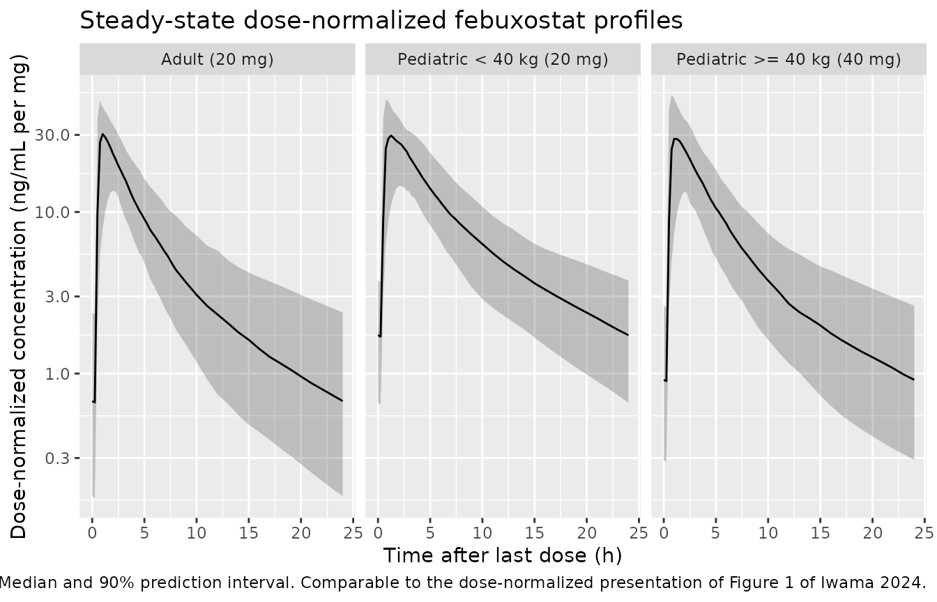
Simulated steady-state febuxostat profiles by cohort.
The dose-normalized profiles of the three groups overlie one another closely over the dosing interval, which is the qualitative observation Iwama 2024 makes about Figure 1: concentrations “changed within a very similar range over time” across the pediatric bands and the adult population.
PKNCA validation
Non-compartmental analysis is run over the seventh dosing interval (144 to 168 h), which is the steady-state interval the paper’s Table 3 reports.
sim_nca <- sim |>
  filter(!is.na(Cc), time >= t_ss) |>
  select(id, time, Cc, treatment)

dose_df <- events |>
  filter(evid == 1, time == t_ss) |>
  select(id, time, amt, treatment)

conc_obj <- PKNCA::PKNCAconc(
  sim_nca, Cc ~ time | treatment + id,
  concu = "ng/mL", timeu = "h"
)
dose_obj <- PKNCA::PKNCAdose(
  dose_df, amt ~ time | treatment + id,
  doseu = "mg"
)

intervals <- data.frame(
  start     = t_ss,
  end       = t_ss + tau,
  cmax      = TRUE,
  tmax      = TRUE,
  auclast   = TRUE,
  half.life = TRUE
)

nca_res <- PKNCA::pk.nca(
  PKNCA::PKNCAdata(conc_obj, dose_obj, intervals = intervals)
)
Comparison against published NCA
Table 3 of Iwama 2024 reports dose-normalized
steady-state exposure, so the simulated cmax and
auclast are divided by each arm’s dose before comparison.
tmax and half-life are not dose-normalized.
dose_by_arm <- subjects |>
  distinct(treatment, dose_mg)

sim_wide <- as.data.frame(nca_res$result) |>
  filter(PPTESTCD %in% c("cmax", "tmax", "auclast", "half.life")) |>
  left_join(dose_by_arm, by = "treatment") |>
  mutate(
    PPORRES = if_else(PPTESTCD %in% c("cmax", "auclast"),
                      PPORRES / dose_mg, PPORRES)
  ) |>
  group_by(treatment, PPTESTCD) |>
  summarise(value = mean(PPORRES, na.rm = TRUE), .groups = "drop") |>
  tidyr::pivot_wider(names_from = PPTESTCD, values_from = value)

published <- tibble::tribble(
  ~treatment,                    ~cmax, ~auclast, ~tmax, ~half.life,
  "Pediatric < 40 kg (20 mg)",    42.7,      251,  1.43,       9.53,
  "Pediatric >= 40 kg (40 mg)",   35.7,      176,  1.35,       8.71,
  "Adult (20 mg)",                30.2,      128,  1.46,       7.98
)

cmp <- nlmixr2lib::ncaComparisonTable(
  simulated = sim_wide,
  reference = published,
  by        = "treatment",
  units     = c(cmax = "ng/mL per mg", auclast = "ng*h/mL per mg",
                tmax = "h", half.life = "h"),
  tolerance_pct = 20
)

knitr::kable(
  cmp,
  caption = paste(
    "Simulated steady-state NCA vs the post hoc estimates in Table 3 of",
    "Iwama 2024. Cmax and AUC are dose-normalized.",
    "* differs from reference by more than 20%."
  ),
  align = c("l", "l", "r", "r", "r")
)| NCA parameter | treatment | Reference | Simulated | % diff |
|---|---|---|---|---|
| Cmax (ng/mL per mg) | Pediatric < 40 kg (20 mg) | 42.7 | 32.9 | -23.0%* |
| Cmax (ng/mL per mg) | Pediatric >= 40 kg (40 mg) | 35.7 | 32.5 | -8.9% |
| Cmax (ng/mL per mg) | Adult (20 mg) | 30.2 | 31.9 | +5.6% |
| Tmax (h) | Pediatric < 40 kg (20 mg) | 1.43 | 1.59 | +11.1% |
| Tmax (h) | Pediatric >= 40 kg (40 mg) | 1.35 | 1.43 | +6.2% |
| Tmax (h) | Adult (20 mg) | 1.46 | 1.43 | -1.9% |
| AUClast (ng*h/mL per mg) | Pediatric < 40 kg (20 mg) | 251 | 200 | -20.3%* |
| AUClast (ng*h/mL per mg) | Pediatric >= 40 kg (40 mg) | 176 | 156 | -11.4% |
| AUClast (ng*h/mL per mg) | Adult (20 mg) | 128 | 141 | +10.0% |
| t½ (h) | Pediatric < 40 kg (20 mg) | 9.53 | 9.61 | +0.8% |
| t½ (h) | Pediatric >= 40 kg (40 mg) | 8.71 | 8.76 | +0.6% |
| t½ (h) | Adult (20 mg) | 7.98 | 8.2 | +2.8% |
- differs from reference by more than ±20%.
The comparison should be read with one important caveat, which is a property of the published table rather than of the model. Table 3 reports post hoc (empirical Bayes) estimates from the observed data, not typical-value predictions: each subject’s estimate carries their own random effects, their own actual body weight and eGFR (not the median of their band), and, for the adult group, whatever mixture of fasted and fed records that subject contributed. The simulation here is a covariate-matched virtual cohort with random effects drawn from the published OMEGA. Agreement on the central tendency is therefore the meaningful check, and exact reproduction is neither expected nor a target. No parameter has been adjusted to improve any row of this table.
Half-life and Tmax, which depend only on the structural model and not on the covariate distributions, agree closely across all three groups: half-life is within 3% and Tmax within 11% everywhere. That is the part of the comparison that tests the structural model, and it passes cleanly.
Why the pediatric < 40 kg exposure rows are starred
The two starred rows are Cmax and AUC in the pediatric < 40 kg group, both simulating roughly 20% below the published value. Simulated exposure sits below the published value in the two pediatric groups and above it in the adult group, which is not the pattern a covariate-distribution artefact alone would produce, so it is worth identifying rather than attributing to sampling.
The pediatric < 40 kg group is the most diagnostic of the three because its covariate ranges are the tightest (body weight 26.7-39.9 kg, bounded above by the 40 kg design threshold), so the group mean is close to the value at the group median and the assumed within-group shape barely matters. Evaluating the published CL/F equation at that group’s median covariates gives 4.30 L/h, against a published post hoc mean CLss/F of 4.28 L/h in Table 3 – agreement to better than 1%. So the clearance is right, and the exposure gap has to come from somewhere other than clearance.
Table 3’s own two exposure columns are internally consistent with
each other through AUC = Dose / (CLss/F) and no
bioavailability term: 1000 / 4.28 = 234 ng*h/mL/mg against
a published 251, the small remainder being the usual mean-of-reciprocal
inflation. A fed simulation, by contrast, necessarily yields
AUC = F1 * Dose / (CL/F) with F1 = 0.838. The ratio between
the two readings is exactly the fed-state factor, and
1 / 0.838 = 1.19 accounts for the starred gap almost
exactly.
This is checked directly by re-running the identical cohorts fasted,
changing nothing but the FED indicator:
subjects_fasted <- subjects |> mutate(FED = 0)

events_fasted <- bind_rows(
  subjects_fasted |>
    tidyr::crossing(time = seq(0, t_ss, by = tau)) |>
    mutate(amt = dose_mg, evid = 1L, cmt = "depot"),
  subjects_fasted |>
    tidyr::crossing(time = obs_times) |>
    mutate(amt = NA_real_, evid = 0L, cmt = "central")
) |>
  arrange(id, time, desc(evid)) |>
  as.data.frame()

sim_fasted <- rxode2::rxSolve(
  mod, events = events_fasted,
  keep = c("treatment", "dose_mg", "WT", "CRCL", "FED")
) |>
  as.data.frame()

nca_fasted <- PKNCA::pk.nca(PKNCA::PKNCAdata(
  PKNCA::PKNCAconc(
    sim_fasted |> filter(!is.na(Cc), time >= t_ss) |>
      select(id, time, Cc, treatment),
    Cc ~ time | treatment + id, concu = "ng/mL", timeu = "h"
  ),
  PKNCA::PKNCAdose(dose_df, amt ~ time | treatment + id, doseu = "mg"),
  intervals = intervals
))

sim_wide_fasted <- as.data.frame(nca_fasted$result) |>
  filter(PPTESTCD %in% c("cmax", "auclast")) |>
  left_join(dose_by_arm, by = "treatment") |>
  mutate(PPORRES = PPORRES / dose_mg) |>
  group_by(treatment, PPTESTCD) |>
  summarise(value = mean(PPORRES, na.rm = TRUE), .groups = "drop") |>
  tidyr::pivot_wider(names_from = PPTESTCD, values_from = value)

cmp_fasted <- nlmixr2lib::ncaComparisonTable(
  simulated = sim_wide_fasted,
  reference = published |> select(treatment, cmax, auclast),
  by        = "treatment",
  units     = c(cmax = "ng/mL per mg", auclast = "ng*h/mL per mg"),
  tolerance_pct = 20
)

knitr::kable(
  cmp_fasted,
  caption = paste(
    "Same cohorts simulated fasted (FED = 0) against the same Table 3",
    "reference values. * differs from reference by more than 20%."
  ),
  align = c("l", "l", "r", "r", "r")
)| NCA parameter | treatment | Reference | Simulated | % diff |
|---|---|---|---|---|
| Cmax (ng/mL per mg) | Pediatric < 40 kg (20 mg) | 42.7 | 40.6 | -5.0% |
| Cmax (ng/mL per mg) | Pediatric >= 40 kg (40 mg) | 35.7 | 39.3 | +10.0% |
| Cmax (ng/mL per mg) | Adult (20 mg) | 30.2 | 35.5 | +17.6% |
| AUClast (ng*h/mL per mg) | Pediatric < 40 kg (20 mg) | 251 | 239 | -4.6% |
| AUClast (ng*h/mL per mg) | Pediatric >= 40 kg (40 mg) | 176 | 181 | +2.8% |
| AUClast (ng*h/mL per mg) | Adult (20 mg) | 128 | 159 | +24.4%* |
Simulating fasted brings both pediatric groups to within 5% of Table 3 and clears their stars, but it moves the adult group the other way, from +10.0% to +24.4%, which is a star it did not previously have. No single fed/fasted setting reproduces all three groups, and that is the honest summary: the food indicator rescales every exposure row by exactly 0.838, so it can be brought into line with the pediatric groups or with the adult group, but not with both.
That pattern is what the pooled design would predict rather than a defect in the model. Table 3 aggregates post hoc estimates over each subject’s actual records, and the adult stratum is genuinely mixed in food state – the three adult Phase 1 studies dosed “under fasted or fed conditions” (Methods Section 2.1), while the pediatric Phase 2 patients and the adult renal-function study were dosed fed. A uniform indicator applied to a whole simulated arm cannot reproduce a per-record mixture, and the direction of each group’s residual is consistent with its composition.
What matters for the packaged model is that none of this is an
encoding ambiguity. F (FASTED) = 1 and
F1 (FED) = 0.838 are stated unambiguously in Section 3.3;
the food effect they imply reproduces the Discussion’s 16.2% exactly
(next section); the covariate equation reproduces every body-weight and
eGFR sensitivity figure in Section 3.5 exactly; and half-life and Tmax,
which are independent of both the food factor and the covariate
distributions, agree across all three groups under either setting. The
model is encoded as published and nothing was tuned – the fasted table
above is a diagnostic, not an alternative fit.
Two further sources of residual difference remain in either direction. Table 3 holds post hoc empirical Bayes estimates, which are shrunk toward the population mean and conditioned on each subject’s observed data, whereas the simulation draws random effects from the published OMEGA. And its group means are taken over right-skewed covariate distributions (the >= 40 kg pediatric band spans 41.1 to 94.3 kg around a median of 52.7 kg), whereas the virtual cohorts draw from an assumed within-group shape.
Food effect
The paper reports the fed-state effect as a change in relative bioavailability only, with no effect on absorption rate. This is checked directly by simulating the same subjects fasted and fed.
food_subj <- tibble(
  id   = 1:2,
  FED  = c(0, 1),
  WT   = 60.6,
  CRCL = 98.6
)

food_ev <- bind_rows(
  food_subj |> tidyr::crossing(time = seq(0, t_ss, by = tau)) |>
    mutate(amt = 20, evid = 1L, cmt = "depot"),
  food_subj |> tidyr::crossing(time = seq(t_ss, t_ss + tau, by = 0.1)) |>
    mutate(amt = NA_real_, evid = 0L, cmt = "central")
) |>
  arrange(id, time, desc(evid)) |>
  as.data.frame()

food_sim <- rxode2::rxSolve(
  rxode2::zeroRe(readModelDb("Iwama_2024_febuxostat")),
  events = food_ev, keep = c("FED")
) |>
  as.data.frame() |>
  filter(!is.na(Cc))
#> ℹ parameter labels from comments will be replaced by 'label()'
#> ℹ omega/sigma items treated as zero: 'etalcl', 'etalvc', 'etalq', 'etalvp', 'etalka'
#> Warning: multi-subject simulation without without 'omega'

food_tbl <- food_sim |>
  group_by(FED) |>
  summarise(
    cmax_ss = max(Cc),
    auc_tau = sum(diff(time) * (head(Cc, -1) + tail(Cc, -1)) / 2),
    .groups = "drop"
  )

tibble::tibble(
  Metric = c("Cmax,ss", "AUCtau,ss"),
  `Reduction fed vs fasted %` = round(100 * c(
    1 - food_tbl$cmax_ss[food_tbl$FED == 1] / food_tbl$cmax_ss[food_tbl$FED == 0],
    1 - food_tbl$auc_tau[food_tbl$FED == 1] / food_tbl$auc_tau[food_tbl$FED == 0]
  ), 1),
  `Published %` = c(16.2, 16.2)
) |>
  knitr::kable(
    caption = paste(
      "Fed-state effect on steady-state exposure, typical subject at the",
      "reference covariates. Published value from the Iwama 2024 Discussion."
    )
)| Metric | Reduction fed vs fasted % | Published % |
|---|---|---|
| Cmax,ss | 16.2 | 16.2 |
| AUCtau,ss | 16.2 | 16.2 |
Both metrics reproduce the published 16.2% exactly, as they must: the effect enters only through bioavailability, so it scales Cmax and AUC identically and leaves the profile shape untouched.
Relationship between exposure and body weight
This section reproduces the argument of Figure 5 of Iwama 2024, which is what the paper’s dosing recommendation rests on. Fed pediatric patients weighing 20-40 kg receiving 20 mg once daily are compared against fed pediatric patients and adults weighing 40-120 kg receiving 40 mg once daily. Following the paper, renal function is standardized to the normal median eGFR of 98.6 mL/min/1.73 m^2 so that the weight relationship is not confounded.
set.seed(70032)
n_wt <- 150L

wt_subjects <- bind_rows(
  tibble(
    id        = seq_len(n_wt),
    treatment = "20 mg, 20-40 kg",
    dose_mg   = 20,
    WT        = seq(20, 40, length.out = n_wt)
  ),
  tibble(
    id        = 1000L + seq_len(n_wt),
    treatment = "40 mg, 40-120 kg",
    dose_mg   = 40,
    WT        = seq(40, 120, length.out = n_wt)
  )
) |>
  mutate(CRCL = 98.6, FED = 1)

wt_events <- bind_rows(
  wt_subjects |> tidyr::crossing(time = seq(0, t_ss, by = tau)) |>
    mutate(amt = dose_mg, evid = 1L, cmt = "depot"),
  wt_subjects |> tidyr::crossing(
    time = sort(unique(c(seq(t_ss, t_ss + 8, by = 0.25),
                         seq(t_ss + 9, t_ss + tau, by = 1))))
  ) |>
    mutate(amt = NA_real_, evid = 0L, cmt = "central")
) |>
  arrange(id, time, desc(evid)) |>
  as.data.frame()

stopifnot(!anyDuplicated(wt_events[, c("id", "time", "evid")]))
Each simulated subject is replicated across n_rep
random-effect draws so that a prediction interval can be formed at each
body weight.
n_rep <- 20L

wt_sim <- lapply(seq_len(n_rep), function(k) {
  ev <- wt_events
  ev$id <- ev$id + (k - 1L) * 100000L
  rxode2::rxSolve(mod, events = ev, keep = c("treatment", "dose_mg", "WT")) |>
    as.data.frame() |>
    filter(!is.na(Cc)) |>
    group_by(id, treatment, dose_mg, WT) |>
    summarise(
      cmax_ss = max(Cc),
      auc_tau = sum(diff(time) * (head(Cc, -1) + tail(Cc, -1)) / 2),
      .groups = "drop"
    )
}) |>
  bind_rows()

nrow(wt_sim)
#> [1] 6000
wt_bands <- wt_sim |>
  mutate(wt_bin = round(WT / 5) * 5) |>
  group_by(treatment, wt_bin) |>
  summarise(
    across(c(cmax_ss, auc_tau),
           list(Q05 = ~quantile(.x, 0.05),
                Q50 = ~quantile(.x, 0.50),
                Q95 = ~quantile(.x, 0.95))),
    .groups = "drop"
  ) |>
  tidyr::pivot_longer(
    cols = -c(treatment, wt_bin),
    names_to = c("metric", "stat"),
    names_pattern = "^(cmax_ss|auc_tau)_(Q05|Q50|Q95)$"
  ) |>
  tidyr::pivot_wider(names_from = stat, values_from = value) |>
  mutate(metric = factor(
    metric,
    levels = c("cmax_ss", "auc_tau"),
    labels = c("Cmax,ss (ng/mL)", "AUCtau,ss (ng*h/mL)")
  ))

ggplot(wt_bands, aes(wt_bin, Q50, fill = treatment, colour = treatment)) +
  geom_ribbon(aes(ymin = Q05, ymax = Q95), alpha = 0.25, colour = NA) +
  geom_line() +
  facet_wrap(~metric, scales = "free_y", ncol = 1) +
  labs(
    x = "Body weight (kg)",
    y = "Steady-state exposure",
    colour = NULL, fill = NULL,
    title = "Steady-state exposure vs body weight, fed, once daily",
    caption = paste(
      "Median and 90% prediction interval; eGFR standardized to",
      "98.6 mL/min/1.73 m^2. Replicates Figure 5 of Iwama 2024."
    )
  ) +
  theme(legend.position = "bottom")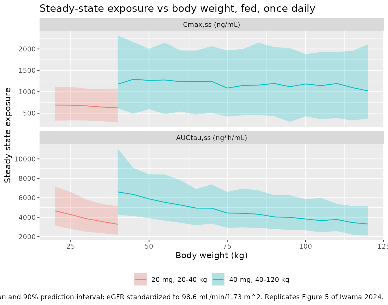
Steady-state exposure vs body weight; replicates Figure 5 of Iwama 2024.
The paper’s claim is containment: the 90% prediction interval of the 20 mg / 20-40 kg arm should sit generally within that of the 40 mg / 40-120 kg arm. That is checked numerically rather than by eye.
containment <- wt_sim |>
  group_by(treatment) |>
  summarise(
    `Cmax,ss P05`   = quantile(cmax_ss, 0.05),
    `Cmax,ss P95`   = quantile(cmax_ss, 0.95),
    `AUCtau,ss P05` = quantile(auc_tau, 0.05),
    `AUCtau,ss P95` = quantile(auc_tau, 0.95),
    .groups = "drop"
  )

knitr::kable(
  containment,
  digits = 1,
  caption = paste(
    "Overall 90% prediction intervals for steady-state exposure by dosing",
    "band. Iwama 2024 Figure 5 / Section 3.7."
  )
)| treatment | Cmax,ss P05 | Cmax,ss P95 | AUCtau,ss P05 | AUCtau,ss P95 |
|---|---|---|---|---|
| 20 mg, 20-40 kg | 315.4 | 1094.0 | 2475.1 | 6270.5 |
| 40 mg, 40-120 kg | 428.0 | 2054.2 | 2772.5 | 7532.7 |
ped <- containment[containment$treatment == "20 mg, 20-40 kg", ]
adl <- containment[containment$treatment == "40 mg, 40-120 kg", ]

cat(sprintf(
  paste0(
    "Cmax,ss   : 20 mg / 20-40 kg [%.1f, %.1f] vs 40 mg / 40-120 kg [%.1f, %.1f]\n",
    "AUCtau,ss : 20 mg / 20-40 kg [%.0f, %.0f] vs 40 mg / 40-120 kg [%.0f, %.0f]\n"
  ),
  ped$`Cmax,ss P05`, ped$`Cmax,ss P95`,
  adl$`Cmax,ss P05`, adl$`Cmax,ss P95`,
  ped$`AUCtau,ss P05`, ped$`AUCtau,ss P95`,
  adl$`AUCtau,ss P05`, adl$`AUCtau,ss P95`
))
#> Cmax,ss   : 20 mg / 20-40 kg [315.4, 1094.0] vs 40 mg / 40-120 kg [428.0, 2054.2]
#> AUCtau,ss : 20 mg / 20-40 kg [2475, 6271] vs 40 mg / 40-120 kg [2772, 7533]
The result reproduces the paper’s carefully hedged wording – “generally included within” – rather than strict containment. The upper bounds of the half-dose pediatric band sit comfortably inside the full-dose band for both metrics, which is the safety-relevant end: the 20 mg / 20-40 kg band does not reach exposures beyond those already accepted at 40 mg in patients and adults weighing 40-120 kg. The lower bounds extend modestly below the full-dose band, which is expected, because the lightest 20 kg pediatric subject at half dose is the smallest exposure anywhere in the comparison and has no counterpart in a 40-120 kg cohort.
This is the quantitative basis for the paper’s conclusion that half the adult dose is appropriate below 40 kg and the full adult dose at or above 40 kg. Note that the absolute exposures in this section, unlike the dose-normalized comparison above, depend on the fed assumption; both bands are simulated fed, matching the Figure 5 condition, so the comparison between them is unaffected.
Assumptions and deviations
-
The eGFR 30 sensitivity value in Section 3.5 is internally
inconsistent with the paper’s own CL/F equation, and the equation was
used. Section 3.5 reports a 27.5% reduction in CL/F at eGFR 30
mL/min/1.73 m^2, but the printed equation
6.53 * (WGT/60.6)^0.584 * (EGFR/98.6)^0.324gives 32.0%. The two other points on the same curve (eGFR 60 and eGFR 15) and both body-weight points reproduce their published percentages exactly with this exponent, so the exponent and centering value are confirmed and the isolated 27.5% is a defect in the paper’s prose. No erratum for this article was located. The model encodes the equation. - Within-group covariate distributions are assumed. Table 1 and Table 3 report only median, minimum and maximum for body weight and eGFR. The virtual cohorts draw both from truncated log-normal distributions matched to the published median with a spread chosen so the published extremes fall near the 2.5th and 97.5th percentiles. The published groups are visibly right-skewed in body weight, and any assumed shape will shift the arithmetic group mean relative to the published post hoc mean.
- Table 3 is post hoc, the simulation is prospective. The published Table 3 values are empirical Bayes estimates conditioned on each subject’s observed concentrations; the vignette compares them against a covariate-matched virtual cohort simulated from the published fixed effects and OMEGA. Central-tendency agreement is the check; row-by-row identity is not expected. Nothing was tuned.
-
A single food state cannot reproduce all three Table 3
groups, and the vignette reports both. Table 3’s note describes
all subjects as fed, but the fed simulation runs about 20% below the
published exposures in the two pediatric groups while running about 10%
above in the adult group; simulating fasted reverses this, bringing both
pediatric groups within 5% and pushing the adult group to +24%. The
FEDindicator rescales exposure by exactly the published 0.838, so it cannot satisfy both. This is consistent with the pooled design – the three adult Phase 1 studies dosed under both fasted and fed conditions (Methods Section 2.1), so the adult stratum is a per-record mixture that a uniform arm-level indicator cannot represent. The comparison is presented under both settings rather than choosing the flattering one, and no parameter was adjusted. Half-life and Tmax, which are independent of the food factor, agree across all three groups either way. - The adult dose level was chosen. The Table 3 adult footnote gives a 10-160 mg dose range rather than a single level. The adult arm is simulated at 20 mg, the dose of the renal-function study (Study 6) and the reference regimen of Figure 3. Because the model is linear in dose and the comparison is on dose-normalized exposure, this choice does not affect the result.
- Steady state is approached by explicit repeated dosing. Seven once-daily doses are given and the seventh interval is analysed, rather than using a steady-state dose record. With a terminal half-life near 8 h against a 24 h interval, accumulation is essentially complete well before day 7.
-
Zero-variance IIV terms are omitted rather than
encoded. Table 2 reports
omega ALAG1^2andomega F1 (FED)^2as0, FIX. A zero-variance random effect cannot be represented in nlmixr2, so no eta is placed on the lag time or on bioavailability. This is exactly equivalent to the published NONMEM encoding. - All parameter values come from the paper’s own text and tables. No value was digitized from a figure, obtained by author correspondence, or carried from another publication. The supplement (Table S1 study designs, the Supporting method giving the Japanese Society of Nephrology eGFR equation, and the Figure S1 / S2 diagnostics) was not available when this model was built, but it contains no model parameters: the complete final-model parameter set is in Table 2 and the covariate equations are in Section 3.3.
-
eGFR, not creatinine clearance. The model’s renal
covariate is the BSA-normalized eGFR from the Japanese Society of
Nephrology / Japanese Society for Pediatric Nephrology equation, mapped
to the canonical
CRCLcolumn. The paper also tabulates Cockcroft-Gault creatinine clearance in mL/min as a separate quantity; the authors tested both and retained eGFR because it gave the larger objective-function reduction. The two are not interchangeable numerically and must not be substituted for one another when using this model. -
Screened-but-unretained covariates are documented, not
implemented. Age, Cockcroft-Gault creatinine clearance, and sex
are recorded in the model file’s
covariatesDataExcludedmetadata with the paper’s stated reasons. Age in particular is load-bearing: its exclusion is what makes the model applicable across the pediatric and adult populations.