PSA disease progression under leuprorelin (Zou 2020)
Source:vignettes/articles/Zou_2020_leuprorelin.Rmd
Zou_2020_leuprorelin.RmdThe model
Zou et al. (2020) built a population disease-progression model of
serum prostate-specific antigen (PSA) in 264 men with hormone-sensitive
prostate cancer who were treated with the LHRH agonist leuprorelin,
using a US medical claims database (Humana, 2007-2011). Two resistance
mechanisms were compared; the final model is the paper’s “clonal
selection” Model II (AIC 295.7 against 865.4 for the “adaptation” Model
I), which splits the observed baseline PSA (PSA_BL)
into
- a drug-resistant fraction
R = exp(-RP)that grows first-order atGRfrom the baseline draw onwards (stategrowth), and - a drug-sensitive fraction
1 - Rthat grows first-order atGSuntil the first leuprorelin dose and is killed first-order atDSfrom then on (stateshrink).
PSA = growth + shrink, so PSA(0) = PSA_BL
exactly. Hemoglobin enters as a power covariate on RP,
baseline PSA as a power covariate on DS, and antiandrogen
use within 30 days of leuprorelin initiation as an exponential covariate
on DS.
This is a disease-progression model with no pharmacokinetics:
leuprorelin enters only through the per-subject time of its first dose,
T_SCAN_TO_DOSE, measured from the baseline PSA draw. There
is therefore no PKNCA section – there is no drug
concentration for non-compartmental analysis to act on. Validation is
structural (closed-form and covariate identities) plus a reproduction of
the paper’s own simulated nadir, time to nadir and PSA-progression
rates.
mod_fun <- readModelDb("Zou_2020_leuprorelin")
mod <- rxode2::rxode2(mod_fun)
#> ℹ parameter labels from comments will be replaced by 'label()'
mod
#>  ── rxode2-based free-form 2-cmt ODE model ──────────────────────────────────────
#>  ── Initalization: ──
#> Fixed Effects ($theta):
#>               lkse          lkge_sens                lrp               lkge
#>          -3.275446          -6.234811           1.371181          -7.332403
#>           e_hgb_rp       e_psa_bl_kse e_antiandrogen_kse              expSd
#>           2.300000           0.174000           0.677000           0.201000
#>
#> Omega ($omega):
#>              etalkse etalkge_sens etalrp etalkge
#> etalkse        0.453         0.00  0.000    0.00
#> etalkge_sens   0.000         2.59  0.000    0.00
#> etalrp         0.000         0.00  0.944    0.00
#> etalkge        0.000         0.00  0.000    3.76
#> attr(,"lotriLabels")
#> [1] "Table 2: omega^2 DS = 0.453"
#> [2] "Table 2: omega^2 GS = 2.59"
#> [3] "Table 2: omega^2 RP = 0.944"
#> [4] "Table 2: omega^2 'DR' = 3.76 (the IIV of GR; the row label is a typo)"
#> attr(,"lotriFix")
#>              etalkse etalkge_sens etalrp etalkge
#> etalkse        FALSE        FALSE  FALSE   FALSE
#> etalkge_sens   FALSE        FALSE  FALSE   FALSE
#> etalrp         FALSE        FALSE  FALSE   FALSE
#> etalkge        FALSE        FALSE  FALSE   FALSE
#>
#> States ($state or $stateDf):
#>   Compartment Number Compartment Name
#> 1                  1           growth
#> 2                  2           shrink
#>  ── μ-referencing ($muRefTable): ──
#>       theta          eta level
#> 1      lkse      etalkse    id
#> 2 lkge_sens etalkge_sens    id
#> 3       lrp       etalrp    id
#> 4      lkge      etalkge    id
#>
#>  ── Model (Normalized Syntax): ──
#> function() {
#>     compartmentData <- list(growth = list(analyte = "PSA", units = "ng/mL",
#>         specimen = "serum", verified = TRUE), shrink = list(analyte = "PSA",
#>         units = "ng/mL", specimen = "serum", verified = TRUE))
#>     covariateData <- list(PSA_BL = list(description = "Observed baseline serum PSA, the last PSA measured before the first leuprorelin dose; the model's time origin is the date of this draw.",
#>         units = "ng/mL", type = "continuous", reference_category = NULL,
#>         source_name = "BAS", notes = "Two roles, both from the paper. (a) It is a per-subject regressor, NOT an estimated parameter, and scales both sub-states (Methods Eqs 2-3): growth(0) = R * PSA_BL and shrink(0) = (1 - R) * PSA_BL, so PSA(0) = PSA_BL exactly. (b) Power covariate on the drug kill rate DS, centered at the cohort median 8.5 ng/mL (Results Eq 17; Table 2 'BAS on DS' = 0.174). Cohort (Table 1): median 8.50 ng/mL, range 0.200-782. Subjects whose baseline PSA was undetectable were excluded (Methods, Study subjects)."),
#>         HGB = list(description = "Baseline blood hemoglobin concentration.",
#>             units = "g/dL", type = "continuous", reference_category = NULL,
#>             source_name = "HGB", notes = "Power covariate on RP, the log-scale parameter of the resistant fraction R = exp(-RP), centered at the cohort median 13.6 g/dL (Results Eq 16; Table 2 'HGB on RP' = 2.30). Lower hemoglobin gives a smaller RP and therefore a LARGER drug-resistant fraction: typical R = 9.36%, 1.94% and 0.326% at the cohort 5th percentile (10.9 g/dL), median (13.6) and 95th percentile (16.0) (Results). Cohort (Table 1): median 13.6 g/dL, range 6.80-17.4. Subjects with hemoglobin < 6 g/dL were excluded as likely acutely ill (Methods)."),
#>         CONMED_ANTIANDROGEN = list(description = "Antiandrogen use indicator: 1 = an antiandrogen (bicalutamide, enzalutamide, flutamide or nilutamide) was dispensed within 30 days of leuprorelin initiation, 0 = not.",
#>             units = "(binary)", type = "binary", reference_category = "0 (no antiandrogen within 30 days of leuprorelin initiation; 231 of 264 subjects)",
#>             source_name = "AND (IND_AND in Eq 17)", notes = "Exponential covariate on DS: DS * exp(0.677 * CONMED_ANTIANDROGEN) (Results Eq 17; Table 2 'AND on DS' = 0.677), i.e. a 96.8% higher kill rate with antiandrogen use (Results). The paper presumes these short courses were given to prevent the testosterone flare of LHRH-agonist initiation (Methods). PSA observed after the start of CONTINUOUS antiandrogen therapy was excluded from the dataset, so this indicator describes a peri-initiation course only. The class composition (bicalutamide, enzalutamide, flutamide, nilutamide) is this paper's definition. Cohort (Table 1): 33 yes, 231 no."),
#>         T_SCAN_TO_DOSE = list(description = "Per-subject time from the baseline PSA draw (the model's time origin) to the first leuprorelin dose.",
#>             units = "day", type = "continuous", reference_category = NULL,
#>             source_name = "t1 (time of the first LHRH dose)",
#>             notes = "Enters as the switch point of the drug-sensitive sub-state (Methods Eqs 2-3): t_s = min(t, t1) and t_k = max(0, t - t1). Before t1 the sensitive clone grows at GS; from t1 onwards it is killed at DS. The resistant clone grows at GR from time 0 regardless. Only the FIRST dose matters: once started, treatment is assumed to act continuously whether the subject was on continuous or intermittent leuprorelin, which the claims data could not distinguish (Discussion, limitations). Dose amount and dose intensity did not enter the model (dose intensity was tested and was not significant). Per-subject DATA from the claims pharmacy fill dates; the paper does not report its distribution."))
#>     covariatesDataExcluded <- list(AGE = list(description = "Age at baseline.",
#>         units = "years", type = "continuous", notes = "Tested in the full covariate model (WAM-BE backward elimination) and not retained. Cohort median 80 years (range 60-100; Table 1)."),
#>         AST = list(description = "Aspartate aminotransferase.",
#>             units = "IU/L", type = "continuous", notes = "Tested and not retained. Cohort median 20 IU/L (range 9-91; Table 1)."),
#>         ALT = list(description = "Alanine aminotransferase.",
#>             units = "IU/L", type = "continuous", notes = "Tested and not retained. Cohort median 18 IU/L (range 4-110; Table 1)."),
#>         CREAT = list(description = "Serum creatinine.", units = "mg/dL",
#>             type = "continuous", notes = "Tested and not retained. Cohort median 1.10 mg/dL (range 0.700-9.30; Table 1)."),
#>         ALP = list(description = "Alkaline phosphatase.", units = "IU/L",
#>             type = "continuous", notes = "Tested and not retained. Cohort median 76.5 IU/L (range 23.0-3640; Table 1)."),
#>         ALB = list(description = "Serum albumin.", units = "g/dL",
#>             type = "continuous", notes = "Tested and not retained. Cohort median 4.13 g/dL (range 2.90-4.80; Table 1)."))
#>     description <- "Population disease-progression model of serum prostate-specific antigen (PSA) in men with hormone-sensitive prostate cancer treated with the LHRH agonist leuprorelin, developed from a US medical claims database (Humana, 2007-2011; 264 subjects, 1113 PSA observations). The final 'clonal selection' structure (the paper's Model II) splits the observed baseline PSA into a drug-resistant fraction R = exp(-RP) that grows first-order at GR from the baseline draw onwards, and a drug-sensitive fraction (1 - R) that grows first-order at GS until the first leuprorelin dose and is then killed first-order at DS. Covariates: hemoglobin (power, on RP), baseline PSA (power, on DS) and antiandrogen use within 30 days of leuprorelin initiation (exponential, on DS). There is no PK input; treatment enters only through the per-subject time of the first leuprorelin dose, T_SCAN_TO_DOSE. Additive residual error on log PSA."
#>     population <- list(species = "human", n_subjects = 264, n_observations = 1113,
#>         n_studies = 1, age_range = "60-100 years (median 80)",
#>         sex_female_pct = 0, race_ethnicity = c(Caucasian = 189,
#>             Black = 59, `Hispanic/other` = 16), regions = "United States (Humana commercially insured; South 196, Midwest 42, West 20, Northeast 6)",
#>         disease_state = "Malignant, hormone-sensitive prostate cancer (ICD-9-CM 185 / ICD-10-CM C61) on leuprorelin as the only LHRH agonist",
#>         dose_range = "Leuprorelin, continuous or intermittent, at any dose; dose intensity (dose received relative to an expected 7.5 mg per month) was not a significant covariate",
#>         baseline_psa = "median 8.50 ng/mL (range 0.200-782)",
#>         baseline_hgb = "median 13.6 g/dL (range 6.80-17.4)",
#>         antiandrogen_use = "33 of 264 within 30 days of leuprorelin initiation",
#>         notes = "Retrospective medical claims data (Humana, 1 January 2007 to 31 December 2011). Inclusion: a PSA before leuprorelin initiation and at least one during treatment. Exclusions (86.4% of eligible patients in total): PSA falling before leuprorelin, undetectable baseline PSA or same-day duplicate measurements; undetectable PSA throughout treatment; incomplete demographics; hemoglobin < 6 g/dL. PSA observations after the start of continuous antiandrogen therapy, surgery, radiotherapy or chemotherapy (whichever first) were dropped. PSA below 0.1 ng/mL (LLOQ) was retained as censored (M3-type likelihood). Estimation: NONMEM 7.3, MCPEM; covariate selection by Wald's approximation with backward elimination (WAM-BE).")
#>     reference <- "Zou Y, Tang F, Talbert JC, Ng CM. Using medical claims database to develop a population disease progression model for leuprorelin-treated subjects with hormone-sensitive prostate cancer. PLoS ONE. 2020;15(3):e0230571. doi:10.1371/journal.pone.0230571. PMCID: PMC7092991. Structural equations from Methods Eqs 2-3 (Model II), IIV form from Eq 4, residual error from Eq 5, covariate forms from Eqs 16-17; all final parameter values from Table 2."
#>     units <- list(time = "day", dosing = "n/a (no PK input; leuprorelin treatment enters only through the per-subject start time T_SCAN_TO_DOSE)",
#>         concentration = "ng/mL (the observable `PSA` is serum prostate-specific antigen)")
#>     vignette <- "Zou_2020_leuprorelin"
#>     ini({
#>         lkse <- -3.2754461763566
#>         label("Kill rate DS of the drug-sensitive PSA fraction after leuprorelin start (1/day)")
#>         lkge_sens <- -6.23481080573971
#>         label("Growth rate GS of the drug-sensitive PSA fraction before leuprorelin start (1/day)")
#>         lrp <- 1.37118072330984
#>         label("RP, minus the log of the drug-resistant fraction R = exp(-RP) (unitless)")
#>         lkge <- -7.33240320650708
#>         label("Growth rate GR of the drug-resistant PSA fraction (1/day)")
#>         e_hgb_rp <- 2.3
#>         label("Power exponent of hemoglobin (/13.6 g/dL) on RP (unitless)")
#>         e_psa_bl_kse <- 0.174
#>         label("Power exponent of baseline PSA (/8.5 ng/mL) on DS (unitless)")
#>         e_antiandrogen_kse <- 0.677
#>         label("Exponential coefficient of antiandrogen use on DS (unitless)")
#>         expSd <- c(0, 0.201)
#>         label("Additive residual error SD on log PSA (log ng/mL)")
#>         etalkse ~ 0.453
#>         label("Table 2: omega^2 DS = 0.453")
#>         etalkge_sens ~ 2.59
#>         label("Table 2: omega^2 GS = 2.59")
#>         etalrp ~ 0.944
#>         label("Table 2: omega^2 RP = 0.944")
#>         etalkge ~ 3.76
#>         label("Table 2: omega^2 'DR' = 3.76 (the IIV of GR; the row label is a typo)")
#>     })
#>     model({
#>         kse <- exp(lkse + etalkse) * (PSA_BL/8.5)^e_psa_bl_kse *
#>             exp(e_antiandrogen_kse * CONMED_ANTIANDROGEN)
#>         kge_sens <- exp(lkge_sens + etalkge_sens)
#>         rp <- exp(lrp + etalrp) * (HGB/13.6)^e_hgb_rp
#>         kge <- exp(lkge + etalkge)
#>         fres <- exp(-rp)
#>         dosed <- time >= T_SCAN_TO_DOSE
#>         d/dt(growth) <- kge * growth
#>         d/dt(shrink) <- (kge_sens * (1 - dosed) - kse * dosed) *
#>             shrink
#>         growth(0) <- fres * PSA_BL
#>         shrink(0) <- (1 - fres) * PSA_BL
#>         PSA <- growth + shrink
#>         PSA ~ lnorm(expSd)
#>     })
#> }
Population
str(mod$meta$population)
#> List of 14
#>  $ species         : chr "human"
#>  $ n_subjects      : num 264
#>  $ n_observations  : num 1113
#>  $ n_studies       : num 1
#>  $ age_range       : chr "60-100 years (median 80)"
#>  $ sex_female_pct  : num 0
#>  $ race_ethnicity  : Named num [1:3] 189 59 16
#>   ..- attr(*, "names")= chr [1:3] "Caucasian" "Black" "Hispanic/other"
#>  $ regions         : chr "United States (Humana commercially insured; South 196, Midwest 42, West 20, Northeast 6)"
#>  $ disease_state   : chr "Malignant, hormone-sensitive prostate cancer (ICD-9-CM 185 / ICD-10-CM C61) on leuprorelin as the only LHRH agonist"
#>  $ dose_range      : chr "Leuprorelin, continuous or intermittent, at any dose; dose intensity (dose received relative to an expected 7.5"| __truncated__
#>  $ baseline_psa    : chr "median 8.50 ng/mL (range 0.200-782)"
#>  $ baseline_hgb    : chr "median 13.6 g/dL (range 6.80-17.4)"
#>  $ antiandrogen_use: chr "33 of 264 within 30 days of leuprorelin initiation"
#>  $ notes           : chr "Retrospective medical claims data (Humana, 1 January 2007 to 31 December 2011). Inclusion: a PSA before leupror"| __truncated__
The 264 subjects (Table 1) had a median age of 80 years (60-100): 189 Caucasian, 59 Black and 16 Hispanic/other, mostly from the US South (196). Median baseline PSA was 8.50 ng/mL (0.200-782) and median hemoglobin 13.6 g/dL (6.80-17.4); 33 subjects received an antiandrogen within 30 days of starting leuprorelin. Patients with a falling pre-treatment PSA, an undetectable baseline or on-treatment PSA, incomplete demographics or hemoglobin below 6 g/dL were excluded, and PSA observed after the start of continuous antiandrogen therapy, surgery, radiotherapy or chemotherapy was dropped. PSA below 0.1 ng/mL (the LLOQ) was retained as censored.
Source trace
trace <- tibble::tribble(
  ~Item, ~Value, ~Source,
  "Model II resistant clone", "PSA_R = BAS * R * exp(GR * t)", "Methods, Eq 2",
  "Model II sensitive clone", "PSA_S = BAS * (1 - R) * exp(GS * t_s) * exp(-DS * t_k)", "Methods, Eq 3",
  "Time split", "t_s = min(t, t1); t_k = max(0, t - t1)", "Methods, text after Eq 3",
  "Resistant fraction", "R = exp(-RP)", "Methods, text after Eq 3",
  "IIV form", "theta_i = theta_typical * exp(eta_i), all parameters", "Methods, Eq 4",
  "Residual error", "additive on log PSA", "Methods, Eq 5; Results",
  "Covariate on RP", "RP = theta_RP * (HGB / 13.6)^theta_HGB_RP", "Results, Eq 16",
  "Covariates on DS", "DS = theta_DS * (BAS / 8.5)^theta_BAS_DS * exp(IND_AND * theta_AND_DS)", "Results, Eq 17",
  "lkse (DS)", "3.78e-2 1/day", "Table 2",
  "lkge_sens (GS)", "1.96e-3 1/day", "Table 2",
  "lrp (RP)", "3.94", "Table 2",
  "lkge (GR)", "6.54e-4 1/day", "Table 2",
  "etalkse", "omega^2 = 0.453", "Table 2",
  "etalkge_sens", "omega^2 = 2.59", "Table 2",
  "etalrp", "omega^2 = 0.944", "Table 2",
  "etalkge", "omega^2 = 3.76 (row labelled 'DR')", "Table 2",
  "e_hgb_rp", "2.30", "Table 2",
  "e_psa_bl_kse", "0.174", "Table 2",
  "e_antiandrogen_kse", "0.677", "Table 2",
  "expSd", "0.201", "Table 2"
)
knitr::kable(trace)| Item | Value | Source |
|---|---|---|
| Model II resistant clone | PSA_R = BAS * R * exp(GR * t) | Methods, Eq 2 |
| Model II sensitive clone | PSA_S = BAS * (1 - R) * exp(GS * t_s) * exp(-DS * t_k) | Methods, Eq 3 |
| Time split | t_s = min(t, t1); t_k = max(0, t - t1) | Methods, text after Eq 3 |
| Resistant fraction | R = exp(-RP) | Methods, text after Eq 3 |
| IIV form | theta_i = theta_typical * exp(eta_i), all parameters | Methods, Eq 4 |
| Residual error | additive on log PSA | Methods, Eq 5; Results |
| Covariate on RP | RP = theta_RP * (HGB / 13.6)^theta_HGB_RP | Results, Eq 16 |
| Covariates on DS | DS = theta_DS * (BAS / 8.5)^theta_BAS_DS * exp(IND_AND * theta_AND_DS) | Results, Eq 17 |
| lkse (DS) | 3.78e-2 1/day | Table 2 |
| lkge_sens (GS) | 1.96e-3 1/day | Table 2 |
| lrp (RP) | 3.94 | Table 2 |
| lkge (GR) | 6.54e-4 1/day | Table 2 |
| etalkse | omega^2 = 0.453 | Table 2 |
| etalkge_sens | omega^2 = 2.59 | Table 2 |
| etalrp | omega^2 = 0.944 | Table 2 |
| etalkge | omega^2 = 3.76 (row labelled ‘DR’) | Table 2 |
| e_hgb_rp | 2.30 | Table 2 |
| e_psa_bl_kse | 0.174 | Table 2 |
| e_antiandrogen_kse | 0.677 | Table 2 |
| expSd | 0.201 | Table 2 |
Structural checks
The ODE form reproduces the published closed form
The model writes Eqs 2-3 as two first-order ODEs whose
sensitive-clone rate switches from +GS to -DS
at T_SCAN_TO_DOSE. Solving it for a stochastic cohort with
a spread of treatment-start delays and comparing each subject’s PSA
against Eqs 2-3 evaluated at the same drawn parameters checks the
encoding. Both sides use identical parameters, so the difference is
numerical error only and a tight bound applies.
set.seed(2020)
n_cf <- 50
cf_cov <- tibble(
  id = seq_len(n_cf),
  PSA_BL = exp(rnorm(n_cf, log(8.5), 1)),
  HGB = rnorm(n_cf, 13.6, 1.5),
  CONMED_ANTIANDROGEN = rbinom(n_cf, 1, 0.125),
  T_SCAN_TO_DOSE = sample(c(0, 14, 45, 90), n_cf, replace = TRUE)
)
cf_times <- c(0, 7, 14, 30, 45, 60, 90, 120, 180, 270, 365, 540, 730)
cf_ev <- tidyr::crossing(cf_cov, time = cf_times) |>
  mutate(evid = 0, amt = 0) |>
  arrange(id, time)

rxode2::rxSetSeed(2020)
cf_sim <- rxode2::rxSolve(
  mod, cf_ev,
  keep = c("PSA_BL", "T_SCAN_TO_DOSE"),
  returnType = "data.frame",
  atol = 1e-10, rtol = 1e-10
)

cf_chk <- cf_sim |>
  mutate(
    t_s = pmin(time, T_SCAN_TO_DOSE),
    t_k = pmax(0, time - T_SCAN_TO_DOSE),
    psa_closed = PSA_BL * fres * exp(kge * time) +
      PSA_BL * (1 - fres) * exp(kge_sens * t_s) * exp(-kse * t_k),
    abs_err = abs(PSA - psa_closed),
    # Extreme etas start some resistant clones near 1e-6 ng/mL, comparable
    # to the solver's absolute tolerance, and the ODE then carries a relative
    # error of order 1e-5 as that clone grows. A structural error (a wrong
    # rate, a missed switch) would be off by tens of percent, so a 1e-4
    # relative bound, plus a small absolute term for near-zero values, still
    # isolates the encoding from numerical noise.
    within = abs_err <= 1e-4 * psa_closed + 1e-8
  )
summary(cf_chk$abs_err / cf_chk$psa_closed)
#>     Min.  1st Qu.   Median     Mean  3rd Qu.     Max.
#> 0.000000 0.000000 0.000000 0.002371 0.000000 1.289103
stopifnot(all(cf_chk$within))
Typical covariate effects match the Results
The Results quote typical RP (and the implied
R) at the cohort 5th percentile, median and 95th percentile
of hemoglobin, and typical DS at the same percentiles of
baseline PSA. These are deterministic functions of Table 2.
th <- mod$theta
rp_typ <- function(hgb) exp(th[["lrp"]]) * (hgb / 13.6)^th[["e_hgb_rp"]]
ds_typ <- function(bas, and = 0) {
  exp(th[["lkse"]]) * (bas / 8.5)^th[["e_psa_bl_kse"]] *
    exp(th[["e_antiandrogen_kse"]] * and)
}
cov_tab <- tibble(
  Quantity = c(
    "RP, HGB 10.9", "RP, HGB 13.6", "RP, HGB 16.0",
    "R (%), HGB 10.9", "R (%), HGB 13.6", "R (%), HGB 16.0",
    "DS (1/day), PSA_BL 0.515", "DS (1/day), PSA_BL 8.5", "DS (1/day), PSA_BL 120",
    "DS increase with antiandrogen (%)",
    "GS doubling time (day)", "GR doubling time (day)"
  ),
  Model = c(
    rp_typ(c(10.9, 13.6, 16.0)),
    100 * exp(-rp_typ(c(10.9, 13.6, 16.0))),
    ds_typ(c(0.515, 8.5, 120)),
    100 * (ds_typ(8.5, 1) / ds_typ(8.5, 0) - 1),
    log(2) / exp(th[["lkge_sens"]]),
    log(2) / exp(th[["lkge"]])
  ),
  Paper = c(
    2.37, 3.94, 5.73, 9.36, 1.94, 0.326,
    2.32e-2, 3.78e-2, 5.99e-2, 96.8, 354, 1060
  )
) |>
  mutate(`Difference (%)` = 100 * (Model / Paper - 1))
knitr::kable(cov_tab, digits = 4)| Quantity | Model | Paper | Difference (%) |
|---|---|---|---|
| RP, HGB 10.9 | 2.3683 | 2.37e+00 | -0.0715 |
| RP, HGB 13.6 | 3.9400 | 3.94e+00 | 0.0000 |
| RP, HGB 16.0 | 5.7258 | 5.73e+00 | -0.0741 |
| R (%), HGB 10.9 | 9.3639 | 9.36e+00 | 0.0420 |
| R (%), HGB 13.6 | 1.9448 | 1.94e+00 | 0.2485 |
| R (%), HGB 16.0 | 0.3261 | 3.26e-01 | 0.0274 |
| DS (1/day), PSA_BL 0.515 | 0.0232 | 2.32e-02 | 0.0321 |
| DS (1/day), PSA_BL 8.5 | 0.0378 | 3.78e-02 | 0.0000 |
| DS (1/day), PSA_BL 120 | 0.0599 | 5.99e-02 | 0.0285 |
| DS increase with antiandrogen (%) | 96.7965 | 9.68e+01 | -0.0036 |
| GS doubling time (day) | 353.6465 | 3.54e+02 | -0.0999 |
| GR doubling time (day) | 1059.8581 | 1.06e+03 | -0.0134 |
All agree to the three significant figures the paper prints.
Virtual cohort and simulated PSA profiles
The cohort draws covariates to match Table 1: baseline PSA log-normal with median 8.5 ng/mL and the 5th/95th percentiles (0.515 / 120 ng/mL) the Results quote; hemoglobin normal with median 13.6 g/dL and the quoted 5th/95th percentiles (10.9 / 16.0 g/dL), truncated to the observed range; antiandrogen use with probability 33/264. The paper does not report the delay from the baseline draw to the first dose, so leuprorelin starts at time 0.
set.seed(71)
n_sub <- 200
bl_sdlog <- (log(120) - log(0.515)) / (2 * qnorm(0.95))
hgb_sd <- (16.0 - 10.9) / (2 * qnorm(0.95))
cohort <- tibble(
  id = seq_len(n_sub),
  PSA_BL = pmin(pmax(exp(rnorm(n_sub, log(8.5), bl_sdlog)), 0.2), 782),
  HGB = pmin(pmax(rnorm(n_sub, 13.6, hgb_sd), 6.8), 17.4),
  CONMED_ANTIANDROGEN = rbinom(n_sub, 1, 33 / 264),
  T_SCAN_TO_DOSE = 0
)
obs_times <- c(0, seq(7, 1095, by = 14))
ev <- tidyr::crossing(cohort, time = obs_times) |>
  mutate(evid = 0, amt = 0) |>
  arrange(id, time)

rxode2::rxSetSeed(71)
sim <- rxode2::rxSolve(mod, ev, returnType = "data.frame")
sim |>
  group_by(time) |>
  summarise(
    q05 = quantile(PSA, 0.05), q50 = median(PSA), q95 = quantile(PSA, 0.95),
    .groups = "drop"
  ) |>
  ggplot(aes(time / 30.4375, q50)) +
  geom_ribbon(aes(ymin = q05, ymax = q95), alpha = 0.25) +
  geom_line() +
  geom_hline(yintercept = 0.1, linetype = "dotted", colour = "blue") +
  scale_y_log10() +
  labs(x = "Time since leuprorelin start (months)", y = "PSA (ng/mL)")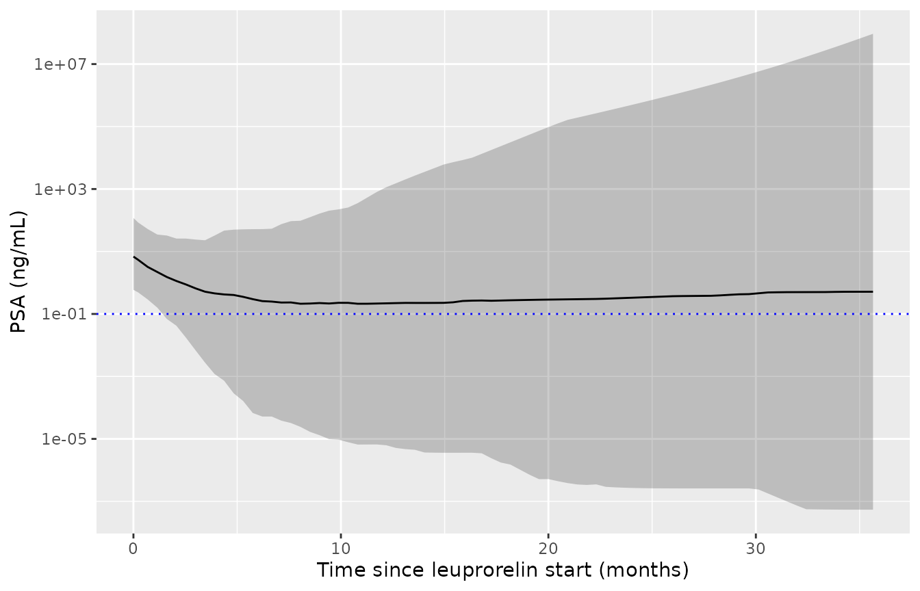
Simulated PSA (individual predictions) in 200 virtual subjects starting leuprorelin at time 0: median with 5th-95th percentile band. The observed-data counterpart is the prediction-corrected VPC of S2 Fig of Zou 2020.
arch <- tibble(
  id = 1:3, HGB = c(10.9, 13.6, 16.0), PSA_BL = 8.5,
  CONMED_ANTIANDROGEN = 0, T_SCAN_TO_DOSE = 60
) |>
  tidyr::crossing(time = seq(0, 1095, by = 5)) |>
  mutate(evid = 0, amt = 0) |>
  arrange(id, time)
arch_sim <- rxode2::rxSolve(rxode2::zeroRe(mod), arch, keep = "HGB", returnType = "data.frame")
#> ℹ omega/sigma items treated as zero: 'etalkse', 'etalkge_sens', 'etalrp', 'etalkge'
#> Warning: multi-subject simulation without without 'omega'
arch_sim |>
  select(time, HGB, Total = PSA, Sensitive = shrink, Resistant = growth) |>
  pivot_longer(c(Total, Sensitive, Resistant), names_to = "part", values_to = "psa") |>
  ggplot(aes(time / 30.4375, psa, colour = part)) +
  geom_line() +
  geom_vline(xintercept = 60 / 30.4375, linetype = "dashed", colour = "red") +
  facet_wrap(~ paste("HGB", HGB, "g/dL")) +
  scale_y_log10() +
  labs(x = "Time since baseline PSA (months)", y = "PSA (ng/mL)", colour = NULL)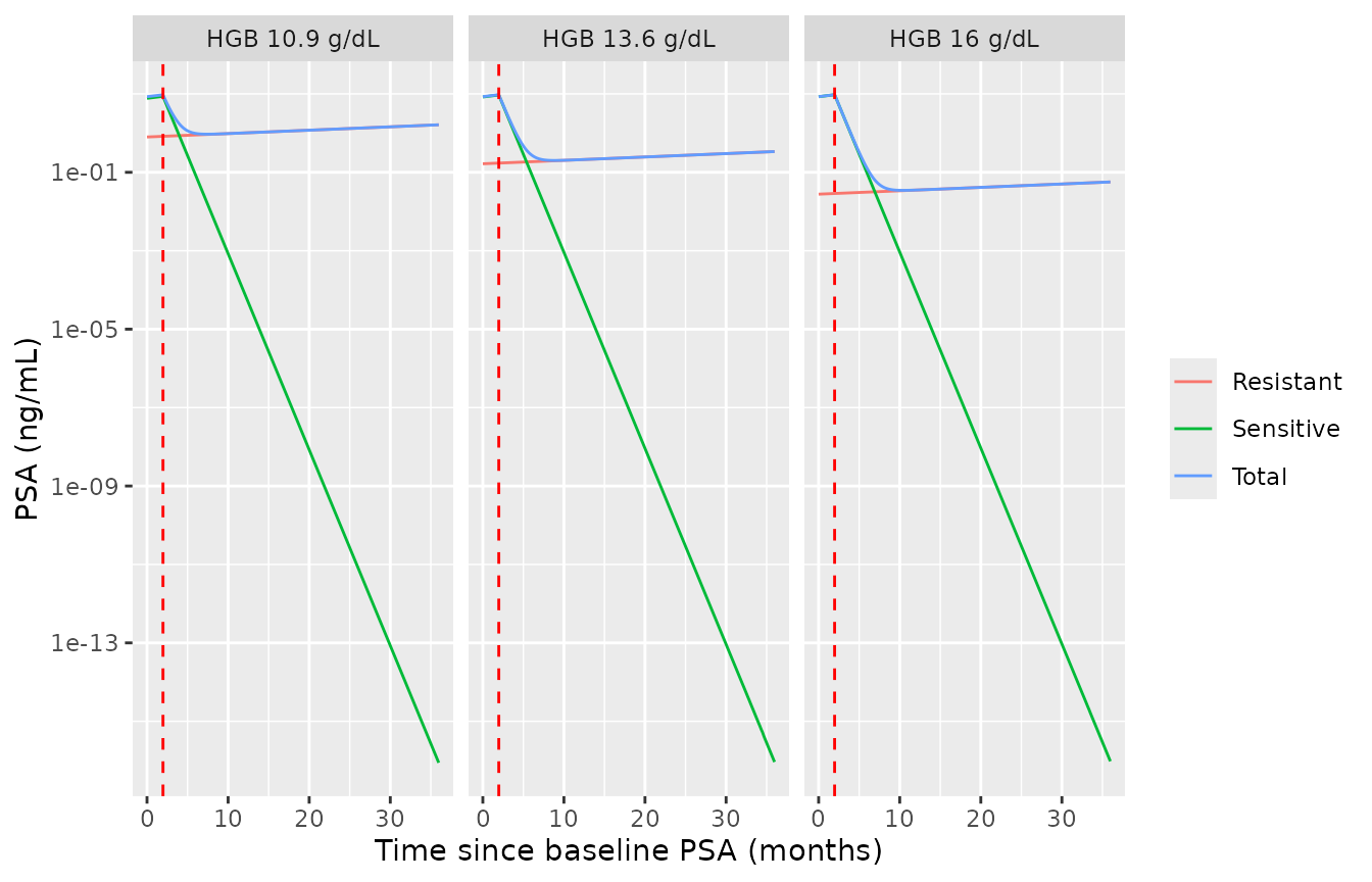
Typical-subject PSA split into its drug-sensitive and drug-resistant parts at the 5th percentile, median and 95th percentile of hemoglobin, with leuprorelin starting 60 days after the baseline draw. Compare the decomposition shown for individual subjects in Figure 4 of Zou 2020.
Reproducing the paper’s simulations
The paper simulated 1000 subjects per scenario at the 5th percentile, median and 95th percentile of one continuous covariate (the others at their medians, no antiandrogen), or with and without antiandrogen, and reported
- the median PSA nadir and median time to nadir (Discussion), and
- the percentage of subjects with PSA progression by PCWG criteria – a rise of at least 25% and at least 2 ng/mL above the nadir, confirmed three or more weeks later – within one, two and three years of starting leuprorelin (Figure 3 and Results).
The simulated quantities below are individual predictions
(between-subject variability, no residual error) on a daily grid, with
treatment starting at time 0. After the nadir each individual prediction
rises monotonically, so any first crossing of the PCWG threshold is
automatically confirmed three weeks later. Because the closed-form check
above shows the ODE and Eqs 2-3 agree, the scenarios are evaluated with
the closed form directly from the packaged model’s theta
and omega, which allows 4000 draws per scenario at
negligible cost.
om <- mod$omega
eta_names <- c("etalkse", "etalkge_sens", "etalrp", "etalkge")
sim_scenario <- function(n, hgb = 13.6, bas = 8.5, and = 0, days = 0:1095) {
  # The four etas are uncorrelated (diagonal omega, Table 2).
  eta <- vapply(eta_names, function(nm) rnorm(n, 0, sqrt(om[nm, nm])), numeric(n))
  kse <- ds_typ(bas, and) * exp(eta[, "etalkse"])
  rp <- rp_typ(hgb) * exp(eta[, "etalrp"])
  kge <- exp(th[["lkge"]] + eta[, "etalkge"])
  fres <- exp(-rp)
  psa <- bas * (fres * exp(outer(kge, days)) + (1 - fres) * exp(-outer(kse, days)))
  nadir <- apply(psa, 1, min)
  t_nadir <- days[apply(psa, 1, which.min)]
  thr <- pmax(1.25 * nadir, nadir + 2)
  t_prog <- vapply(seq_len(n), function(i) {
    j <- which(psa[i, ] >= thr[i] & days > t_nadir[i])
    if (length(j) > 0) days[j[1]] else Inf
  }, numeric(1))
  tibble(
    nadir = median(nadir), t_nadir = median(t_nadir),
    p1 = 100 * mean(t_prog <= 365), p2 = 100 * mean(t_prog <= 730),
    p3 = 100 * mean(t_prog <= 1095)
  )
}
set.seed(354)
scen <- tibble::tribble(
  ~Scenario, ~hgb, ~bas, ~and,
  "HGB 10.9 g/dL", 10.9, 8.5, 0,
  "Median covariates", 13.6, 8.5, 0,
  "HGB 16.0 g/dL", 16.0, 8.5, 0,
  "PSA_BL 0.515 ng/mL", 13.6, 0.515, 0,
  "PSA_BL 120 ng/mL", 13.6, 120, 0,
  "Antiandrogen use", 13.6, 8.5, 1
)
scen_res <- scen |>
  rowwise() |>
  mutate(res = list(sim_scenario(4000, hgb, bas, and))) |>
  ungroup() |>
  tidyr::unnest(res)
paper_prog <- tibble::tribble(
  ~Scenario, ~p1_paper, ~p3_paper,
  "HGB 10.9 g/dL", 19.8, 38.8,
  "Median covariates", 13.9, 28.2,
  "HGB 16.0 g/dL", 10.5, 22.1,
  "PSA_BL 0.515 ng/mL", 6.9, 15.8,
  "PSA_BL 120 ng/mL", 25.6, 47.8,
  "Antiandrogen use", NA, 28.5
)
prog_cmp <- scen_res |>
  left_join(paper_prog, by = "Scenario") |>
  select(Scenario, p1, p1_paper, p2, p3, p3_paper)
prog_cmp |>
  dplyr::rename(
    "Progression by 1 y (%), simulated" = p1,
    "Progression by 1 y (%), paper" = p1_paper,
    "Progression by 2 y (%), simulated" = p2,
    "Progression by 3 y (%), simulated" = p3,
    "Progression by 3 y (%), paper" = p3_paper
  ) |>
knitr::kable(digits = 1)| Scenario | Progression by 1 y (%), simulated | Progression by 1 y (%), paper | Progression by 2 y (%), simulated | Progression by 3 y (%), simulated | Progression by 3 y (%), paper |
|---|---|---|---|---|---|
| HGB 10.9 g/dL | 18.2 | 19.8 | 28.7 | 35.8 | 38.8 |
| Median covariates | 13.7 | 13.9 | 22.2 | 28.0 | 28.2 |
| HGB 16.0 g/dL | 10.1 | 10.5 | 17.6 | 22.4 | 22.1 |
| PSA_BL 0.515 ng/mL | 6.0 | 6.9 | 11.2 | 15.2 | 15.8 |
| PSA_BL 120 ng/mL | 25.9 | 25.6 | 39.4 | 46.1 | 47.8 |
| Antiandrogen use | 14.3 | NA | 22.9 | 29.1 | 28.5 |
Replicates Figure 3 of Zou 2020. The two-year percentages are shown in Figure 3 but not quoted numerically in the text, so they have no paper column.
d1 <- prog_cmp$p1 - prog_cmp$p1_paper
d3 <- prog_cmp$p3 - prog_cmp$p3_paper
stopifnot(
  # Every quoted rate within 5 percentage points (the paper's own Monte Carlo
  # standard error at n = 1000 is about 1.5 points at these rates).
  all(abs(d1) < 5, na.rm = TRUE),
  all(abs(d3) < 5, na.rm = TRUE),
  # The covariate orderings the paper reports.
  with(scen_res, p3[Scenario == "HGB 10.9 g/dL"] > p3[Scenario == "Median covariates"]),
  with(scen_res, p3[Scenario == "Median covariates"] > p3[Scenario == "HGB 16.0 g/dL"]),
  with(scen_res, p3[Scenario == "PSA_BL 120 ng/mL"] > p3[Scenario == "Median covariates"]),
  with(scen_res, p3[Scenario == "Median covariates"] > p3[Scenario == "PSA_BL 0.515 ng/mL"])
)
paper_nadir <- tibble::tribble(
  ~Scenario, ~nadir_paper, ~t_nadir_paper,
  "HGB 10.9 g/dL", 1.19, 155,
  "Median covariates", 0.290, 198,
  "HGB 16.0 g/dL", 0.0574, 240,
  "PSA_BL 0.515 ng/mL", 0.0220, 294,
  "PSA_BL 120 ng/mL", 3.47, 135
)
nadir_cmp <- scen_res |>
  inner_join(paper_nadir, by = "Scenario") |>
  select(Scenario, nadir, nadir_paper, t_nadir, t_nadir_paper) |>
  mutate(
    nadir_ratio = nadir / nadir_paper,
    t_nadir_ratio = t_nadir / t_nadir_paper
  )
nadir_cmp |>
  dplyr::rename(
    "Median nadir (ng/mL), simulated" = nadir,
    "Median nadir (ng/mL), paper" = nadir_paper,
    "Median time to nadir (day), simulated" = t_nadir,
    "Median time to nadir (day), paper" = t_nadir_paper,
    "Nadir ratio" = nadir_ratio,
    "Time-to-nadir ratio" = t_nadir_ratio
  ) |>
knitr::kable(digits = 3)| Scenario | Median nadir (ng/mL), simulated | Median nadir (ng/mL), paper | Median time to nadir (day), simulated | Median time to nadir (day), paper | Nadir ratio | Time-to-nadir ratio |
|---|---|---|---|---|---|---|
| HGB 10.9 g/dL | 1.090 | 1.190 | 159.0 | 155 | 0.916 | 1.026 |
| Median covariates | 0.246 | 0.290 | 204.0 | 198 | 0.849 | 1.030 |
| HGB 16.0 g/dL | 0.056 | 0.057 | 244.0 | 240 | 0.976 | 1.017 |
| PSA_BL 0.515 ng/mL | 0.018 | 0.022 | 298.5 | 294 | 0.839 | 1.015 |
| PSA_BL 120 ng/mL | 3.478 | 3.470 | 137.0 | 135 | 1.002 | 1.015 |
stopifnot(
  # The median nadir spans two orders of magnitude across scenarios; its
  # sample median is noisy at the paper's n = 1000, so allow 30%.
  all(abs(log(nadir_cmp$nadir_ratio)) < log(1.3)),
  all(abs(nadir_cmp$t_nadir_ratio - 1) < 0.15)
)
The nadir values reproduce the two-orders-of-magnitude spread the Discussion reports, and time to nadir agrees within about 7%. The simulated median nadir at median covariates (about 0.24-0.25 ng/mL against the quoted 0.290) sits at the low end of the agreement; the sample median of a quantity this skewed moves by tens of percent between Monte Carlo cohorts of 1000.
Assumptions and deviations
-
Row label ‘DR’ in Table 2. The fourth IIV row is
labelled
omega^2 DR; Methods states IIV was estimated on all four structural parameters and there is noDRparameter, so it is taken as the IIV ofGR. -
Table 2 IIV values are variances. The column is
headed
omega^2. The reproduction of the Figure 3 progression rates and the Discussion nadir values confirms the variance reading. -
Residual error. Eq 5 is additive on log PSA,
encoded as
lnorm(expSd)withexpSd = 0.201. The paper retained PSA below the 0.1 ng/mL LLOQ as censored observations; censoring is a property of the data, not the model. - Treatment start. Only the first leuprorelin dose enters the model. The analysis pooled continuous and intermittent regimens (which the claims data could not distinguish), and dose intensity was tested and not retained. The vignette simulations start treatment at time 0 because the paper does not report the baseline-to-first-dose interval.
- Simulation settings for Figure 3. The paper states only that 1000 subjects per scenario were simulated in R with the final model. The reproduction assumes individual predictions without residual error, the non-varied covariates at their medians, no antiandrogen in the continuous covariate scenarios (the median rows of the hemoglobin and baseline-PSA panels are identical, 13.9% and 28.2%, and equal the no-antiandrogen three-year value), and progression timed from the start of leuprorelin. The close agreement supports these readings.
- Covariate cohort. Table 1 gives medians and ranges only; the log-normal baseline-PSA and normal hemoglobin distributions are built from the 5th and 95th percentiles quoted in the Results.
-
Screened but not retained covariates. The
continuous candidates (age, AST, ALT, serum creatinine, alkaline
phosphatase, albumin) are documented in the model file’s
covariatesDataExcluded, not used. Race and region were collected (Methods; Table 1) and are not in the final model; the paper does not give their indicator coding, so they are recorded only in the model’spopulationmetadata.