Tofacitinib in ulcerative colitis (Vong 2021)
Source:vignettes/articles/Vong_2021_tofacitinib.Rmd
Vong_2021_tofacitinib.RmdModel and source
- Citation: Vong C, Martin SW, Deng C, Xie R, Ito K, Su C, Sandborn WJ, Mukherjee A. Population Pharmacokinetics of Tofacitinib in Patients With Moderate to Severe Ulcerative Colitis. Clin Pharmacol Drug Dev. 2021; 10(3): 229-240. doi:10.1002/cpdd.899. PMCID: PMC7986169.
- Description: One-compartment population PK model with first-order absorption and an absorption lag time for oral immediate-release tofacitinib in 1096 adults with moderately to severely active ulcerative colitis, pooled from the phase 2 dose-ranging induction study A3921063, the phase 3 OCTAVE Induction 1 and 2 studies and the phase 3 OCTAVE Sustain maintenance study (Vong 2021). The model is parameterized in apparent oral clearance (CL/F) and apparent volume of distribution (V/F). CL/F varies with baseline creatinine clearance (power 0.354 on CRCL_BASE/108.7) and multiplicative factors for female sex (0.868) and Asian race (0.932); V/F varies with baseline body weight (power 0.585 on WT/72), age (power -0.116 on AGE/40) and female sex (0.845). Inter-individual variability is an exponential eta on CL/F only; V/F has no eta of its own, its individual deviation being the paper’s ‘scaling parameter’ (0.392) times the CL/F eta. Ka carries inter-occasion variability (six occasions, no inter-individual variability). Residual error is proportional (additive on the log scale) with a magnitude that switches on time after dose at 8 hours (41.6% at or before 8 h, 68.9% after), and the residual magnitude itself carries a 58.0% inter-individual variability (etaruv).
- Article: https://doi.org/10.1002/cpdd.899
- Open-access full text: https://www.ncbi.nlm.nih.gov/pmc/articles/PMC7986169/
Tofacitinib is an oral Janus kinase inhibitor approved for ulcerative colitis (UC). Vong 2021 pooled the tofacitinib UC development program – the phase 2 dose-ranging induction study A3921063, the two identical phase 3 induction studies OCTAVE Induction 1 and 2, and the 52-week phase 3 maintenance study OCTAVE Sustain – and fitted a one-compartment model with lagged first-order absorption, parameterized in apparent oral clearance (CL/F) and apparent volume of distribution (V/F). Covariates were selected by stepwise covariate modeling. The final model keeps baseline creatinine clearance, sex and Asian race on CL/F, and body weight, age and sex on V/F.
mod <- rxode2::rxode2(readModelDb("Vong_2021_tofacitinib"))
#> ℹ parameter labels from comments will be replaced by 'label()'
#> Warning: some etas defaulted to non-mu referenced, possible parsing error: etaiov_lka_1, etaiov_lka_2, etaiov_lka_3, etaiov_lka_4, etaiov_lka_5, etaiov_lka_6
#> as a work-around try putting the mu-referenced expression on a simple line
Population
Baseline demographics reproduce Table 2 of Vong 2021 (n = 1096 tofacitinib-treated patients, 7231 plasma concentration records).
| Characteristic | Value |
|---|---|
| Age, years | median 40, mean 41.3 (SD 13.8), range 18-80 |
| Body weight (BWT), kg | median 72, mean 73.6 (SD 16.6), range 37-154.5 |
| Baseline creatinine clearance (BCCL), mL/min | median 108.7, mean 112.3 (SD 30.3), range 40.8-255.2 |
| Female | 41.5% |
| Race | White 81.3%, Asian 10.9%, Other 4.2%, Black 1.0% |
| Baseline total Mayo score | mean 8.9 (SD 1.5), range 3-12 |
| Concomitant 5-ASA / oral corticosteroids | 77.7% / 42.8% |
| Doses | 0.5, 3, 5, 10 or 15 mg twice daily (immediate release) |
Sampling was sparse in the phase 3 studies (a predose sample plus one sample 0.5 h or 2 h after an in-clinic dose, per visit) and serial in the phase 2 study (predose and 0.25, 0.5, 1 and 2-3 h post-dose at baseline and week 8; Table 1). Creatinine clearance below 40 mL/min was an exclusion criterion in every study.
The reference patient used throughout the paper’s covariate assessment (Results; Figure 1 legend) is non-Asian, male, body weight 72.0 kg, age 40.0 years, baseline creatinine clearance 108.7 mL/min – the cohort medians.
reference_patient <- list(
  CRCL_BASE = 108.7, SEXF = 0, RACE_ASIAN = 0, WT = 72, AGE = 40, OCC = 1
)
tau <- 12 # dosing interval, h
Source trace
Every structural parameter, covariate effect and variance component, with the location it was read from. All values are from the printed paper. The supplement (study sites, and two diagnostic figures) carries no parameter values. Figure 1 was digitized from the vector graphic in the article PDF for the forest-plot comparison below; it does not supply any model value.
| Model quantity | Source location | Value |
|---|---|---|
| One-compartment, first-order absorption + lag | Results, Final Model Results | structure |
lka = log(Ka) |
Abstract and Results (9.85 h^-1); Table 3 (9.9, RSE 7.1%) | 9.85 |
lcl = log(CL/F) |
Table 3, CL/F, L/h
|
26.3 (RSE 1.2%) |
lvc = log(V/F) |
Table 3, V/F, L
|
115.8 (RSE 1.1%) |
ltlag = log(lag time) |
Table 3, Lag time, h
|
0.236 (RSE 0.52%) |
| Continuous covariate form | Methods; Results; Table 3 footnote d | power of (cov / median) |
| Categorical covariate form | Table 3 footnote d | fraction of the reference category |
e_crcl_base_cl |
Table 3, CL/F ~ BCCL | 0.354 |
e_sexf_cl |
Table 3, CL/F ~ Female | 0.868 |
e_race_asian_cl |
Table 3, CL/F ~ Asian | 0.932 |
e_wt_vc |
Table 3, V/F ~ Body weight | 0.585 |
e_age_vc |
Table 3, V/F ~ Age | -0.116 |
e_sexf_vc |
Table 3, V/F ~ Female | 0.845 |
| Reference covariate values | Results, Final Model Results | 72.0 kg, 40.0 y, 108.7 mL/min |
etalcl |
Table 3, CL/F IIV column |
22.2% |
vc_eta_scale |
Table 3, Scaling parameter; Equation 1b |
0.392 |
etaiov_lka_1 … etaiov_lka_6
|
Table 3, Ka IOV column; Results (6 occasions) |
191.8% |
etaruv |
Table 3, IIV column on both proportional-error rows | 58.0% |
propSd_early |
Table 3, Proportional error, TAD <= 8 h, %
|
41.6 |
propSd_late |
Table 3, Proportional error, TAD > 8 h, %
|
68.9 |
| Residual error on log scale = proportional | Methods, Data Analysis | form |
| Concentration units (ng/mL) | Methods (LLOQ 0.100 ng/mL); Figure 2 axis | ng/mL |
Three structural points are stated in prose or equations rather than in the table:
-
V/F carries no eta of its own. Equation 1b is
V_i = theta_TV_V * exp(eta_CL,i * theta_scale): the V/F deviation is a fixed multiple (0.392) of the CL/F deviation, which forces the CL/F-V/F random-effect correlation to exactly 1. It is implemented asvc_eta_scale * etalcl. -
Ka has inter-occasion but no inter-individual
variability (“only IOV was included as a random effect on Ka”).
The paper reports shrinkage for “the 6 occasions estimated”, so six
occasion slots sharing one variance are carried, indexed by the
OCCcolumn. -
The residual magnitude has its own inter-individual
variability. Both residual-error rows of Table 3 carry the same
58.0% IIV, i.e. one eta scaling the proportional SD for each subject; it
is carried as
etaruv.
Typical values for the reference patient
The model must return the paper’s point estimates for the reference patient, where every covariate term collapses to 1. The derived elimination half-life is checked against the paper’s 3.05 h.
tv <- rxode2::zeroRe(mod)
#> Warning: No sigma parameters in the model
#> Warning: some etas defaulted to non-mu referenced, possible parsing error: etaiov_lka_1, etaiov_lka_2, etaiov_lka_3, etaiov_lka_4, etaiov_lka_5, etaiov_lka_6
#> as a work-around try putting the mu-referenced expression on a simple line

with_covariates <- function(ev, overrides = list()) {
  p <- utils::modifyList(reference_patient, overrides)
  out <- as.data.frame(ev)
  for (nm in names(p)) out[[nm]] <- p[[nm]]
  out
}

single <- rxode2::et(amt = 10, cmt = "depot") |> rxode2::et(1, cmt = "central")
param_at <- function(overrides, what) {
  rxode2::rxSolve(tv, with_covariates(single, overrides), returnType = "data.frame")[[what]][1]
}

typical <- data.frame(
  Parameter = c("CL/F (L/h)", "V/F (L)", "Ka (1/h)", "Lag time (h)"),
  Model = c(param_at(list(), "cl"), param_at(list(), "vc"),
            param_at(list(), "ka"), param_at(list(), "tlag")),
  Paper = c(26.3, 115.8, 9.85, 0.236)
)
#> ℹ omega/sigma items treated as zero: 'etalcl', 'etaiov_lka_1', 'etaiov_lka_2', 'etaiov_lka_3', 'etaiov_lka_4', 'etaiov_lka_5', 'etaiov_lka_6', 'etaruv'
#> ℹ omega/sigma items treated as zero: 'etalcl', 'etaiov_lka_1', 'etaiov_lka_2', 'etaiov_lka_3', 'etaiov_lka_4', 'etaiov_lka_5', 'etaiov_lka_6', 'etaruv'
#> ℹ omega/sigma items treated as zero: 'etalcl', 'etaiov_lka_1', 'etaiov_lka_2', 'etaiov_lka_3', 'etaiov_lka_4', 'etaiov_lka_5', 'etaiov_lka_6', 'etaruv'
#> ℹ omega/sigma items treated as zero: 'etalcl', 'etaiov_lka_1', 'etaiov_lka_2', 'etaiov_lka_3', 'etaiov_lka_4', 'etaiov_lka_5', 'etaiov_lka_6', 'etaruv'
knitr::kable(typical, digits = 4)| Parameter | Model | Paper |
|---|---|---|
| CL/F (L/h) | 26.300 | 26.300 |
| V/F (L) | 115.800 | 115.800 |
| Ka (1/h) | 9.850 | 9.850 |
| Lag time (h) | 0.236 | 0.236 |
stopifnot(isTRUE(all.equal(typical$Model, typical$Paper, tolerance = 1e-8)))

t_half <- log(2) * param_at(list(), "vc") / param_at(list(), "cl")
#> ℹ omega/sigma items treated as zero: 'etalcl', 'etaiov_lka_1', 'etaiov_lka_2', 'etaiov_lka_3', 'etaiov_lka_4', 'etaiov_lka_5', 'etaiov_lka_6', 'etaruv'
#> ℹ omega/sigma items treated as zero: 'etalcl', 'etaiov_lka_1', 'etaiov_lka_2', 'etaiov_lka_3', 'etaiov_lka_4', 'etaiov_lka_5', 'etaiov_lka_6', 'etaruv'
cat(sprintf("Elimination half-life: %.3f h (paper: approximately 3.05 h)\n", t_half))
#> Elimination half-life: 3.052 h (paper: approximately 3.05 h)
stopifnot(abs(t_half - 3.05) < 0.005)
Reproducing the paper’s covariate-effect statements
The Effect of Covariates section quantifies each covariate effect in prose. These are exact arithmetic checks on deterministic functions of the covariates, so the tolerance is set from the precision each number was printed to.
base_cl <- param_at(list(), "cl")
#> ℹ omega/sigma items treated as zero: 'etalcl', 'etaiov_lka_1', 'etaiov_lka_2', 'etaiov_lka_3', 'etaiov_lka_4', 'etaiov_lka_5', 'etaiov_lka_6', 'etaruv'
base_vc <- param_at(list(), "vc")
#> ℹ omega/sigma items treated as zero: 'etalcl', 'etaiov_lka_1', 'etaiov_lka_2', 'etaiov_lka_3', 'etaiov_lka_4', 'etaiov_lka_5', 'etaiov_lka_6', 'etaruv'

impacts <- dplyr::bind_rows(
  data.frame(Quantity = "CL/F", Scenario = "Female vs male",
             Model = 100 * (param_at(list(SEXF = 1), "cl") / base_cl - 1),
             Paper = -13.2, Tolerance = 0.05),
  data.frame(Quantity = "CL/F", Scenario = "Asian vs non-Asian",
             Model = 100 * (param_at(list(RACE_ASIAN = 1), "cl") / base_cl - 1),
             Paper = -6.8, Tolerance = 0.05),
  # Quoted to the nearest whole percent.
  data.frame(Quantity = "CL/F", Scenario = "BCCL 60 vs 108.7 mL/min",
             Model = 100 * (param_at(list(CRCL_BASE = 60), "cl") / base_cl - 1),
             Paper = -19, Tolerance = 0.5),
  data.frame(Quantity = "V/F", Scenario = "BWT 53 vs 72 kg",
             Model = 100 * (param_at(list(WT = 53), "vc") / base_vc - 1),
             Paper = -16.4, Tolerance = 0.05),
  data.frame(Quantity = "V/F", Scenario = "BWT 95 vs 72 kg",
             Model = 100 * (param_at(list(WT = 95), "vc") / base_vc - 1),
             Paper = 17.6, Tolerance = 0.05),
  data.frame(Quantity = "V/F", Scenario = "Female vs male",
             Model = 100 * (param_at(list(SEXF = 1), "vc") / base_vc - 1),
             Paper = -15.5, Tolerance = 0.05),
  data.frame(Quantity = "V/F", Scenario = "Age 80 vs 40 y",
             Model = 100 * (param_at(list(AGE = 80), "vc") / base_vc - 1),
             Paper = -7.7, Tolerance = 0.05)
) |>
  dplyr::mutate(Difference = Model - Paper, Pass = abs(Difference) < Tolerance)
#> ℹ omega/sigma items treated as zero: 'etalcl', 'etaiov_lka_1', 'etaiov_lka_2', 'etaiov_lka_3', 'etaiov_lka_4', 'etaiov_lka_5', 'etaiov_lka_6', 'etaruv'
#> ℹ omega/sigma items treated as zero: 'etalcl', 'etaiov_lka_1', 'etaiov_lka_2', 'etaiov_lka_3', 'etaiov_lka_4', 'etaiov_lka_5', 'etaiov_lka_6', 'etaruv'
#> ℹ omega/sigma items treated as zero: 'etalcl', 'etaiov_lka_1', 'etaiov_lka_2', 'etaiov_lka_3', 'etaiov_lka_4', 'etaiov_lka_5', 'etaiov_lka_6', 'etaruv'
#> ℹ omega/sigma items treated as zero: 'etalcl', 'etaiov_lka_1', 'etaiov_lka_2', 'etaiov_lka_3', 'etaiov_lka_4', 'etaiov_lka_5', 'etaiov_lka_6', 'etaruv'
#> ℹ omega/sigma items treated as zero: 'etalcl', 'etaiov_lka_1', 'etaiov_lka_2', 'etaiov_lka_3', 'etaiov_lka_4', 'etaiov_lka_5', 'etaiov_lka_6', 'etaruv'
#> ℹ omega/sigma items treated as zero: 'etalcl', 'etaiov_lka_1', 'etaiov_lka_2', 'etaiov_lka_3', 'etaiov_lka_4', 'etaiov_lka_5', 'etaiov_lka_6', 'etaruv'
#> ℹ omega/sigma items treated as zero: 'etalcl', 'etaiov_lka_1', 'etaiov_lka_2', 'etaiov_lka_3', 'etaiov_lka_4', 'etaiov_lka_5', 'etaiov_lka_6', 'etaruv'

impacts |>
  dplyr::rename("Change from model (%)" = Model, "Change reported by paper (%)" = Paper,
                "Difference (pp)" = Difference, "Tolerance (pp)" = Tolerance) |>
knitr::kable(digits = 3)| Quantity | Scenario | Change from model (%) | Change reported by paper (%) | Tolerance (pp) | Difference (pp) | Pass |
|---|---|---|---|---|---|---|
| CL/F | Female vs male | -13.200 | -13.2 | 0.05 | 0.000 | TRUE |
| CL/F | Asian vs non-Asian | -6.800 | -6.8 | 0.05 | 0.000 | TRUE |
| CL/F | BCCL 60 vs 108.7 mL/min | -18.971 | -19.0 | 0.50 | 0.029 | TRUE |
| V/F | BWT 53 vs 72 kg | -16.409 | -16.4 | 0.05 | -0.009 | TRUE |
| V/F | BWT 95 vs 72 kg | 17.606 | 17.6 | 0.05 | 0.006 | TRUE |
| V/F | Female vs male | -15.500 | -15.5 | 0.05 | 0.000 | TRUE |
| V/F | Age 80 vs 40 y | -7.726 | -7.7 | 0.05 | -0.026 | TRUE |
Every statement reproduces to the precision the paper printed.
Steady-state solve against the closed form
A one-compartment oral model with a lag has a closed-form steady-state solution. Both sides use the same parameter values, so they differ only by numerical integration error and a tight bound is appropriate.
n_load <- 28 # 29 doses over 14 days
t_ss <- n_load * tau

# Log-spaced grid: absorption is fast (Ka 9.85 /h), so the peak needs fine early
# resolution, while the trough needs coverage out to 12 h.
obs_times <- sort(unique(c(0, exp(seq(log(0.01), log(tau), length.out = 300)))))

ss_closed_form <- function(t, dose, ka, kel, v, tau, tlag) {
  tt <- (t - tlag) %% tau
  amp <- dose * ka / (v * (ka - kel))
  1000 * amp * (exp(-kel * tt) / (1 - exp(-kel * tau)) -
                  exp(-ka * tt) / (1 - exp(-ka * tau)))
}

ss_profile <- function(dose, overrides = list()) {
  ev <- rxode2::et(amt = dose, cmt = "depot", ii = tau, addl = n_load) |>
    rxode2::et(t_ss + obs_times, cmt = "central")
  rxode2::rxSolve(tv, with_covariates(ev, overrides), returnType = "data.frame",
                  maxsteps = 100000L)
}

cf_check <- lapply(c(5, 10), function(dose) {
  d <- ss_profile(dose)
  cf <- ss_closed_form(d$time - t_ss, dose, d$ka[1], d$cl[1] / d$vc[1], d$vc[1], tau, d$tlag[1])
  data.frame(
    Dose = paste(dose, "mg BID"),
    `Cmax ODE` = max(d$Cc), `Cmax closed form` = max(cf),
    `Cmin ODE` = min(d$Cc), `Cmin closed form` = min(cf),
    `Max relative difference` = max(abs(d$Cc - cf) / cf),
    check.names = FALSE
  )
}) |> dplyr::bind_rows()
#> ℹ omega/sigma items treated as zero: 'etalcl', 'etaiov_lka_1', 'etaiov_lka_2', 'etaiov_lka_3', 'etaiov_lka_4', 'etaiov_lka_5', 'etaiov_lka_6', 'etaruv'
#> ℹ omega/sigma items treated as zero: 'etalcl', 'etaiov_lka_1', 'etaiov_lka_2', 'etaiov_lka_3', 'etaiov_lka_4', 'etaiov_lka_5', 'etaiov_lka_6', 'etaruv'

knitr::kable(cf_check, digits = c(0, 3, 3, 3, 3, 10))| Dose | Cmax ODE | Cmax closed form | Cmin ODE | Cmin closed form | Max relative difference |
|---|---|---|---|---|---|
| 5 mg BID | 42.339 | 42.339 | 3.1 | 3.1 | 9.486e-07 |
| 10 mg BID | 84.679 | 84.679 | 6.2 | 6.2 | 9.253e-07 |
Mass balance: CL/F x AUC(0-tau) = Dose at steady state
Because the model is parameterized in apparent clearance, the
steady-state identity CL/F * AUC(0-tau) = Dose is exact.
For the reference patient at 10 mg twice daily, it gives 10 mg / 26.3
L/h = 380.2 ng*h/mL.
trap <- function(t, y) sum(diff(t) * (head(y, -1) + tail(y, -1)) / 2)

mb_typical <- lapply(c(5, 10), function(dose) {
  d <- ss_profile(dose)
  auc <- trap(d$time, d$Cc)
  data.frame(
    Dose = paste(dose, "mg BID"),
    `AUC(0-tau) simulated (ng*h/mL)` = auc,
    `Dose / (CL/F) (ng*h/mL)` = 1000 * dose / d$cl[1],
    `Relative difference` = abs(auc - 1000 * dose / d$cl[1]) / (1000 * dose / d$cl[1]),
    check.names = FALSE
  )
}) |> dplyr::bind_rows()
#> ℹ omega/sigma items treated as zero: 'etalcl', 'etaiov_lka_1', 'etaiov_lka_2', 'etaiov_lka_3', 'etaiov_lka_4', 'etaiov_lka_5', 'etaiov_lka_6', 'etaruv'
#> ℹ omega/sigma items treated as zero: 'etalcl', 'etaiov_lka_1', 'etaiov_lka_2', 'etaiov_lka_3', 'etaiov_lka_4', 'etaiov_lka_5', 'etaiov_lka_6', 'etaruv'

knitr::kable(mb_typical, digits = c(0, 3, 3, 10))| Dose | AUC(0-tau) simulated (ng*h/mL) | Dose / (CL/F) (ng*h/mL) | Relative difference |
|---|---|---|---|
| 5 mg BID | 190.123 | 190.114 | 4.95282e-05 |
| 10 mg BID | 380.247 | 380.228 | 4.94007e-05 |
The same computation against a deliberately broken copy of the model, whose concentration scale factor is 10-fold wrong, shows the gate can fail.
broken <- rxode2::rxode2(
  paste(
    "cl <- 26.3; vc <- 115.8; ka <- 9.85; tlag <- 0.236; kel <- cl / vc",
    "d/dt(depot) <- -ka * depot",
    "d/dt(central) <- ka * depot - kel * central",
    "alag(depot) <- tlag",
    "Cc <- 10000 * central / vc", # deliberately 10x wrong
    sep = "\n"
  )
)
ev_b <- rxode2::et(amt = 10, cmt = "depot", ii = tau, addl = n_load) |>
  rxode2::et(t_ss + obs_times, cmt = "central")
db <- rxode2::rxSolve(broken, ev_b, returnType = "data.frame", maxsteps = 100000L)
mutation_rel_diff <- abs(trap(db$time, db$Cc) - 10000 / 26.3) / (10000 / 26.3)
cat("Mutated model relative difference:", signif(mutation_rel_diff, 4), "\n")
#> Mutated model relative difference: 9
stopifnot(mutation_rel_diff > 1)
Replicating Figure 1 (covariate impact on AUC and Cmax)
Figure 1 of Vong 2021 is a forest plot of steady-state AUC and Cmax at 10 mg twice daily for each covariate scenario, relative to the reference patient. The point estimates below were digitized by the maintainers from the vector graphic in the article PDF (diamond centres mapped through the 80/100/120/140% axis ticks; the four AUC points that must equal 100% read back as 99.97%, so the reading precision is about 0.1 percentage points). The published confidence intervals come from 1000 nonparametric bootstrap runs and are not reproducible from point estimates.
fig1 <- data.frame(
  Scenario = rep(c("Age 30 y", "Age 80 y", "BWT 53 kg", "BWT 95 kg",
                   "BCCL 60 mL/min", "Female", "Asian"), each = 2),
  Metric = rep(c("AUC", "Cmax"), 7),
  Paper = c(99.97, 97.45, 99.97, 106.37, 99.97, 114.67, 99.97, 89.05,
            123.22, 106.25, 115.08, 117.57, 107.43, 101.92)
)
scenarios <- list(
  "Age 30 y" = list(AGE = 30), "Age 80 y" = list(AGE = 80),
  "BWT 53 kg" = list(WT = 53), "BWT 95 kg" = list(WT = 95),
  "BCCL 60 mL/min" = list(CRCL_BASE = 60), "Female" = list(SEXF = 1),
  "Asian" = list(RACE_ASIAN = 1)
)

ss_metrics <- function(overrides) {
  d <- ss_profile(10, overrides)
  c(AUC = trap(d$time, d$Cc), Cmax = max(d$Cc))
}
ref_metrics <- ss_metrics(list())
#> ℹ omega/sigma items treated as zero: 'etalcl', 'etaiov_lka_1', 'etaiov_lka_2', 'etaiov_lka_3', 'etaiov_lka_4', 'etaiov_lka_5', 'etaiov_lka_6', 'etaruv'
forest <- lapply(names(scenarios), function(nm) {
  m <- ss_metrics(scenarios[[nm]])
  data.frame(Scenario = nm, Metric = c("AUC", "Cmax"),
             Model = 100 * as.numeric(m / ref_metrics))
}) |>
  dplyr::bind_rows() |>
  dplyr::left_join(fig1, by = c("Scenario", "Metric")) |>
  dplyr::mutate(Difference = Model - Paper)
#> ℹ omega/sigma items treated as zero: 'etalcl', 'etaiov_lka_1', 'etaiov_lka_2', 'etaiov_lka_3', 'etaiov_lka_4', 'etaiov_lka_5', 'etaiov_lka_6', 'etaruv'
#> ℹ omega/sigma items treated as zero: 'etalcl', 'etaiov_lka_1', 'etaiov_lka_2', 'etaiov_lka_3', 'etaiov_lka_4', 'etaiov_lka_5', 'etaiov_lka_6', 'etaruv'
#> ℹ omega/sigma items treated as zero: 'etalcl', 'etaiov_lka_1', 'etaiov_lka_2', 'etaiov_lka_3', 'etaiov_lka_4', 'etaiov_lka_5', 'etaiov_lka_6', 'etaruv'
#> ℹ omega/sigma items treated as zero: 'etalcl', 'etaiov_lka_1', 'etaiov_lka_2', 'etaiov_lka_3', 'etaiov_lka_4', 'etaiov_lka_5', 'etaiov_lka_6', 'etaruv'
#> ℹ omega/sigma items treated as zero: 'etalcl', 'etaiov_lka_1', 'etaiov_lka_2', 'etaiov_lka_3', 'etaiov_lka_4', 'etaiov_lka_5', 'etaiov_lka_6', 'etaruv'
#> ℹ omega/sigma items treated as zero: 'etalcl', 'etaiov_lka_1', 'etaiov_lka_2', 'etaiov_lka_3', 'etaiov_lka_4', 'etaiov_lka_5', 'etaiov_lka_6', 'etaruv'
#> ℹ omega/sigma items treated as zero: 'etalcl', 'etaiov_lka_1', 'etaiov_lka_2', 'etaiov_lka_3', 'etaiov_lka_4', 'etaiov_lka_5', 'etaiov_lka_6', 'etaruv'

forest |>
  dplyr::rename("Model (% of reference)" = Model,
                "Figure 1, digitized (% of reference)" = Paper,
                "Difference (pp)" = Difference) |>
knitr::kable(digits = 2)| Scenario | Metric | Model (% of reference) | Figure 1, digitized (% of reference) | Difference (pp) |
|---|---|---|---|---|
| Age 30 y | AUC | 100.00 | 99.97 | 0.03 |
| Age 30 y | Cmax | 97.58 | 97.45 | 0.13 |
| Age 80 y | AUC | 100.00 | 99.97 | 0.03 |
| Age 80 y | Cmax | 106.22 | 106.37 | -0.15 |
| BWT 53 kg | AUC | 100.00 | 99.97 | 0.03 |
| BWT 53 kg | Cmax | 114.71 | 114.67 | 0.04 |
| BWT 95 kg | AUC | 100.00 | 99.97 | 0.03 |
| BWT 95 kg | Cmax | 89.10 | 89.05 | 0.05 |
| BCCL 60 mL/min | AUC | 123.41 | 123.22 | 0.19 |
| BCCL 60 mL/min | Cmax | 106.44 | 106.25 | 0.19 |
| Female | AUC | 115.21 | 115.08 | 0.13 |
| Female | Cmax | 117.53 | 117.57 | -0.04 |
| Asian | AUC | 107.30 | 107.43 | -0.13 |
| Asian | Cmax | 101.94 | 101.92 | 0.02 |
forest_long <- forest |>
  dplyr::select(Scenario, Metric, Model, Paper) |>
  tidyr::pivot_longer(c(Model, Paper), names_to = "Source", values_to = "Ratio")
forest_long$Scenario <- factor(forest_long$Scenario, levels = rev(names(scenarios)))

ggplot(forest_long, aes(x = Ratio, y = Scenario, colour = Metric, shape = Source)) +
  geom_vline(xintercept = 100, colour = "grey40") +
  geom_vline(xintercept = c(80, 125), linetype = 3, colour = "grey60") +
  geom_point(position = position_dodge(width = 0.6), size = 2.4) +
  scale_shape_manual(values = c(Model = 16, Paper = 1),
                     labels = c(Model = "Model", Paper = "Figure 1 (digitized)")) +
  labs(x = "Change relative to the reference patient (%)", y = NULL,
       colour = NULL, shape = NULL) +
  theme_bw() + theme(legend.position = "top")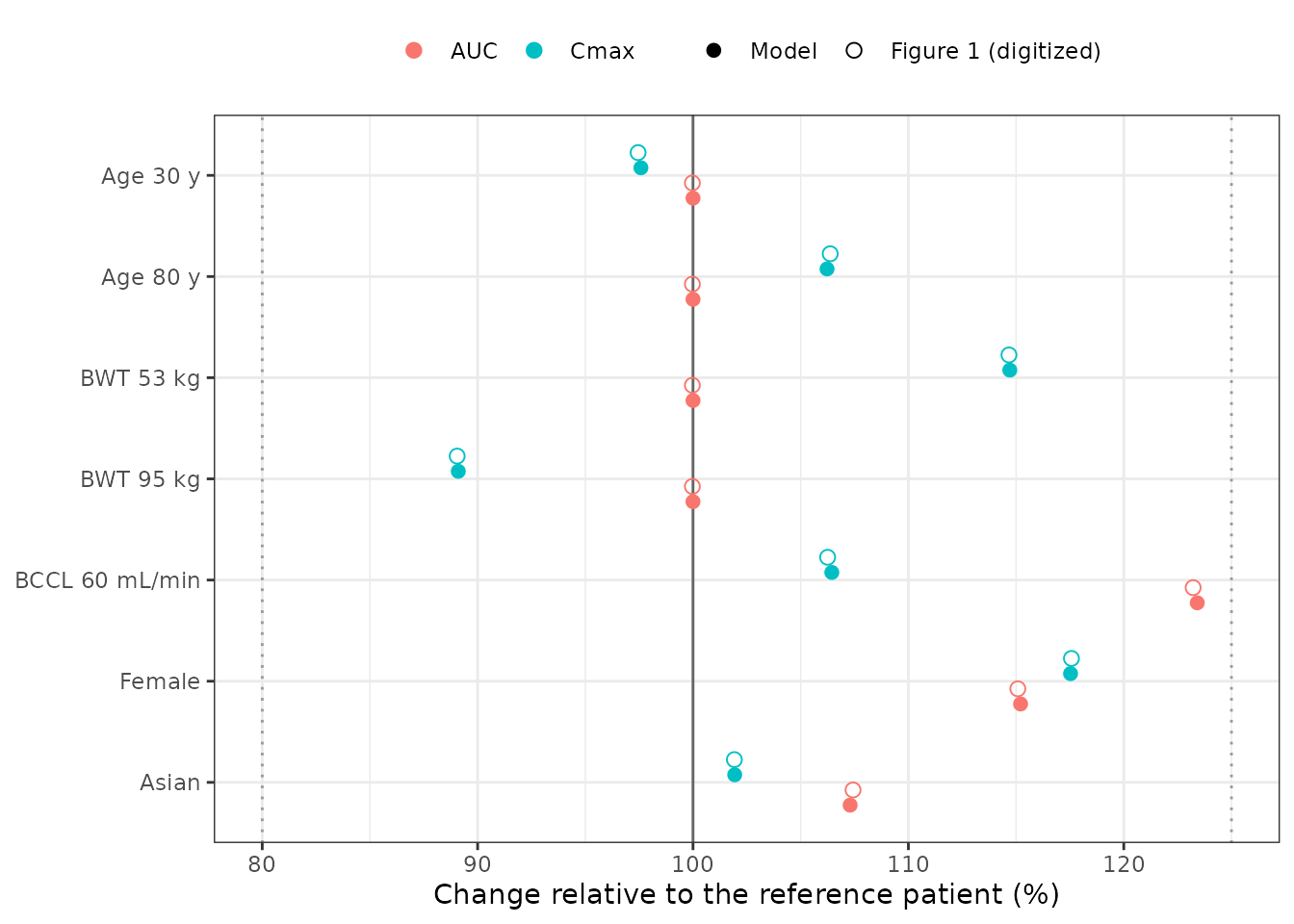
Replicates the point estimates of Figure 1 of Vong 2021: steady-state AUC and Cmax at 10 mg twice daily relative to the reference patient (non-Asian male, 72 kg, 40 years, BCCL 108.7 mL/min). Filled points: model; open points: digitized from the published figure.
All fourteen points agree to within a quarter of a percentage point, which is the digitization precision plus the small offset expected from the paper having plotted bootstrap medians rather than the final-model point estimates. Because the Cmax ratios depend jointly on CL/F, V/F, Ka and the dosing interval, this agreement also confirms the absorption rate and the V/F covariate model, not just the clearance model.
Virtual cohort
200 virtual subjects are drawn with covariate distributions matching Table 2, and each subject is simulated at both 5 and 10 mg twice daily, so the dose-proportionality check below is an exact test of model linearity.
Table 2 reports mean, SD, median and range. The continuous covariates are drawn from normal distributions matched to the reported mean and SD, with any draw outside the reported range rejected and redrawn (the range is a definition of the population, so it is not clamped). The race and sex indicators are drawn independently.
Every record is assigned OCC = 1: the simulation
represents a single steady-state visit, so the occasion-1 Ka eta acts as
that subject’s absorption deviation for the visit.
rxode2::rxSetSeed(20210301)
set.seed(20210301)
n_sub <- 200

rtrunc_norm <- function(n, mean, sd, lower, upper) {
  x <- stats::rnorm(n, mean, sd)
  while (any(bad <- x < lower | x > upper)) {
    x[bad] <- stats::rnorm(sum(bad), mean, sd)
  }
  x
}

cohort <- data.frame(
  id = seq_len(n_sub),
  AGE = rtrunc_norm(n_sub, 41.3, 13.8, 18, 80),
  WT = rtrunc_norm(n_sub, 73.6, 16.6, 37, 154.5),
  CRCL_BASE = rtrunc_norm(n_sub, 112.3, 30.3, 40.8, 255.2),
  SEXF = stats::rbinom(n_sub, 1, 0.415),
  RACE_ASIAN = stats::rbinom(n_sub, 1, 0.109),
  OCC = 1L
)

cohort |>
  dplyr::summarise(
    `Age (y)` = sprintf("%.1f (%.1f)", mean(AGE), sd(AGE)),
    `Weight (kg)` = sprintf("%.1f (%.1f)", mean(WT), sd(WT)),
    `BCCL (mL/min)` = sprintf("%.1f (%.1f)", mean(CRCL_BASE), sd(CRCL_BASE)),
    `Female (%)` = sprintf("%.1f", 100 * mean(SEXF)),
    `Asian (%)` = sprintf("%.1f", 100 * mean(RACE_ASIAN))
  ) |>
  tidyr::pivot_longer(dplyr::everything(), names_to = "Characteristic",
                      values_to = "Simulated cohort, mean (SD) or %") |>
knitr::kable()| Characteristic | Simulated cohort, mean (SD) or % |
|---|---|
| Age (y) | 42.9 (12.4) |
| Weight (kg) | 74.2 (16.5) |
| BCCL (mL/min) | 113.6 (28.8) |
| Female (%) | 46.5 |
| Asian (%) | 10.5 |
The Ka inter-occasion variability is very large (191.8%), so a subject two SDs into the slow tail absorbs with a rate constant of about 0.2 1/h (half-life of absorption about 3.5 h) rather than the typical 4 minutes. The 14-day loading period is sized from that tail, not from the 3-hour elimination half-life, so every subject is at steady state when the NCA interval opens.
Each arm is solved in its own rxSolve() call with the
rxode2 seed reset identically, so subject i receives the
same random-effect draw at both dose levels; the chunk asserts that.
simulate_arm <- function(dose) {
  rxode2::rxSetSeed(20210301)
  events <- do.call(rbind, lapply(cohort$id, function(i) {
    rbind(
      data.frame(id = i, time = 0, amt = dose, evid = 1L,
                 cmt = "depot", ii = tau, addl = n_load),
      data.frame(id = i, time = t_ss + obs_times, amt = NA_real_, evid = 0L,
                 cmt = "central", ii = 0, addl = 0L)
    )
  }))
  events <- dplyr::left_join(events, cohort, by = "id")
  rxode2::rxSolve(mod, events, returnType = "data.frame", maxsteps = 100000L) |>
    dplyr::mutate(dose = dose, treatment = paste(dose, "mg BID"), tad = time - t_ss)
}

sim <- dplyr::bind_rows(simulate_arm(5), simulate_arm(10))
sim$treatment <- factor(sim$treatment, levels = c("5 mg BID", "10 mg BID"))

individual_params <- sim |>
  dplyr::group_by(treatment, id) |>
  dplyr::summarise(cl = dplyr::first(cl), vc = dplyr::first(vc),
                   ka = dplyr::first(ka), .groups = "drop")

p5 <- dplyr::filter(individual_params, treatment == "5 mg BID")
p10 <- dplyr::filter(individual_params, treatment == "10 mg BID")
stopifnot(
  identical(p5$id, p10$id),
  isTRUE(all.equal(p5[, c("cl", "vc", "ka")], p10[, c("cl", "vc", "ka")]))
)
Replicating Figure 2 (visual predictive check by dose)
Figure 2B of Vong 2021 is a prediction-corrected VPC stratified by
dose. The panel below is the simulated counterpart for the two approved
doses over one steady-state dosing interval, using the concentrations
with residual error (sim), whose magnitude switches at 8 h
after dose.
pct <- sim |>
  dplyr::filter(tad > 0) |>
  dplyr::group_by(treatment, tad) |>
  dplyr::summarise(
    p05 = quantile(sim, 0.05), p50 = median(sim), p95 = quantile(sim, 0.95),
    .groups = "drop"
  )

ggplot(pct, aes(x = tad)) +
  geom_ribbon(aes(ymin = p05, ymax = p95), alpha = 0.25, fill = "steelblue") +
  geom_line(aes(y = p50), linewidth = 0.8) +
  facet_wrap(~treatment) +
  scale_y_log10() +
  scale_x_continuous(breaks = seq(0, 12, 2)) +
  labs(x = "Time after dose (hours)", y = "Plasma concentration (ng/mL)") +
  theme_bw()
#> Warning in transformation$transform(x): NaNs produced
#> Warning in scale_y_log10(): log-10 transformation introduced infinite values.
#> Warning: Removed 320 rows containing missing values or values outside the scale range
#> (`geom_ribbon()`).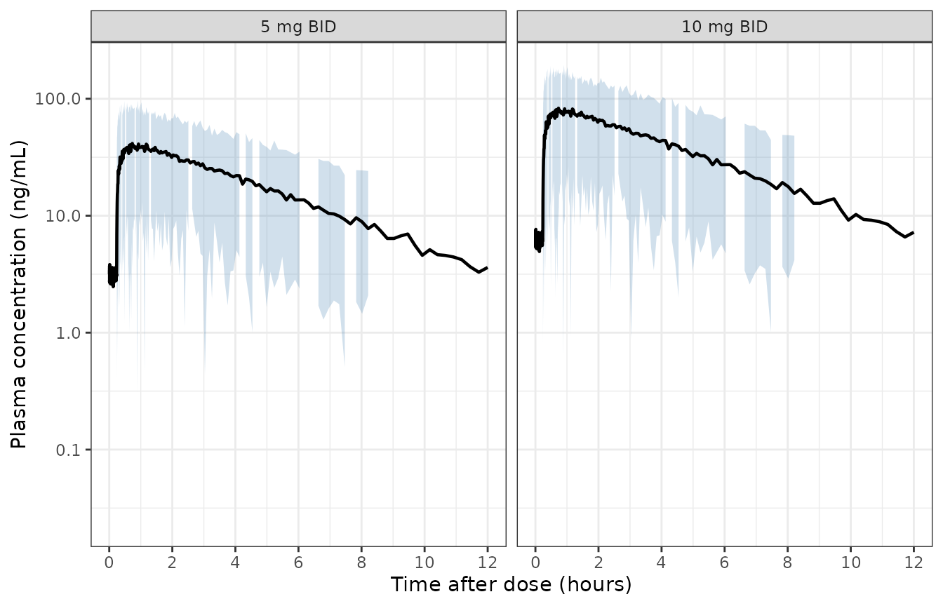
Replicates Figure 2B of Vong 2021 (5 and 10 mg twice-daily strata): simulated 5th, 50th and 95th percentiles of tofacitinib concentration, with residual error, over a steady-state dosing interval.
PKNCA validation at steady state
NCA is run on the structural prediction Cc (no residual
error).
conc_data <- sim |>
  dplyr::filter(!is.na(Cc)) |>
  dplyr::select(id, treatment, time, Cc)

anchor_count <- conc_data |>
  dplyr::filter(time == t_ss) |>
  dplyr::count(treatment, id)
stopifnot(nrow(anchor_count) == 2 * n_sub, all(anchor_count$n == 1))

dose_data <- sim |>
  dplyr::distinct(treatment, id, dose) |>
  dplyr::mutate(time = t_ss)

conc_obj <- PKNCA::PKNCAconc(
  conc_data, Cc ~ time | treatment + id, concu = "ng/mL", timeu = "h"
)
dose_obj <- PKNCA::PKNCAdose(
  dose_data, dose ~ time | treatment + id, route = "extravascular", duration = 0
)

intervals <- data.frame(
  start = t_ss, end = t_ss + tau,
  cmax = TRUE, tmax = TRUE, cmin = TRUE, auclast = TRUE, cav = TRUE
)

nca <- PKNCA::pk.nca(PKNCA::PKNCAdata(conc_obj, dose_obj, intervals = intervals))
nca_res <- as.data.frame(nca$result)
Simulated steady-state exposure
nca_summary <- nca_res |>
  dplyr::filter(PPTESTCD %in% c("cmax", "tmax", "cmin", "auclast", "cav")) |>
  dplyr::group_by(treatment, PPTESTCD) |>
  dplyr::summarise(
    Median = median(PPORRES), P10 = quantile(PPORRES, 0.1),
    P90 = quantile(PPORRES, 0.9), .groups = "drop"
  ) |>
  dplyr::mutate(PPTESTCD = factor(
    PPTESTCD,
    levels = c("cmax", "tmax", "cmin", "cav", "auclast"),
    labels = c("Cmax,ss (ng/mL)", "Tmax (h)", "Cmin,ss (ng/mL)",
               "Cavg,ss (ng/mL)", "AUC(0-tau) (ng*h/mL)")
  )) |>
  dplyr::arrange(treatment, PPTESTCD)

nca_summary |>
  dplyr::rename("Dose group" = treatment, "NCA parameter" = PPTESTCD,
                "10th percentile" = P10, "90th percentile" = P90) |>
knitr::kable(digits = 2)| Dose group | NCA parameter | Median | 10th percentile | 90th percentile |
|---|---|---|---|---|
| 5 mg BID | Cmax,ss (ng/mL) | 44.05 | 31.04 | 57.32 |
| 5 mg BID | Tmax (h) | 0.56 | 0.28 | 2.28 |
| 5 mg BID | Cmin,ss (ng/mL) | 3.35 | 1.37 | 8.44 |
| 5 mg BID | Cavg,ss (ng/mL) | 16.94 | 12.33 | 24.82 |
| 5 mg BID | AUC(0-tau) (ng*h/mL) | 203.29 | 148.02 | 297.79 |
| 10 mg BID | Cmax,ss (ng/mL) | 88.10 | 62.08 | 114.65 |
| 10 mg BID | Tmax (h) | 0.56 | 0.28 | 2.28 |
| 10 mg BID | Cmin,ss (ng/mL) | 6.70 | 2.75 | 16.88 |
| 10 mg BID | Cavg,ss (ng/mL) | 33.88 | 24.67 | 49.63 |
| 10 mg BID | AUC(0-tau) (ng*h/mL) | 406.57 | 296.03 | 595.57 |
Comparison against the published exposure summary
The Effect of Covariates section reports geometric-mean (%CV) steady-state AUC of 211.3 ng*h/mL (22.6%) at 5 mg and 403.8 ng*h/mL (24.6%) at 10 mg twice daily. It then reports geometric-mean “Cmax” of 3.6 ng/mL (47.4%) and 6.7 ng/mL (51.2%). Those two values cannot be peak concentrations. At 10 mg, Dose/V alone is 10 mg / 115.8 L = 86 ng/mL, the reference-patient steady-state Cmax is 85 ng/mL (closed form, above), and the Figure 1 Cmax ratios reproduce to 0.2 percentage points, so the model’s Cmax is the paper’s Cmax. The Methods list four derived exposure metrics: AUC, average concentration, Cmax and trough concentration. The table below compares the printed values with the simulated geometric mean of each candidate quantity.
geo <- function(x) exp(mean(log(x)))
geo_cv <- function(x) 100 * sqrt(exp(stats::var(log(x))) - 1)

simulated_geo <- nca_res |>
  dplyr::filter(PPTESTCD %in% c("auclast", "cmax", "cav", "cmin")) |>
  dplyr::group_by(treatment, PPTESTCD) |>
  dplyr::summarise(value = geo(PPORRES), gcv = geo_cv(PPORRES), .groups = "drop") |>
  dplyr::mutate(treatment = as.character(treatment))
sim_value <- function(trt, what) {
  simulated_geo$value[simulated_geo$treatment == trt & simulated_geo$PPTESTCD == what]
}

printed_c <- c("5 mg BID" = 3.6, "10 mg BID" = 6.7)
elimination <- lapply(names(printed_c), function(trt) {
  data.frame(
    Dose = trt,
    Printed = printed_c[[trt]],
    `Cmax / 10` = sim_value(trt, "cmax") / 10,
    Cavg = sim_value(trt, "cav"),
    Ctrough = sim_value(trt, "cmin"),
    check.names = FALSE
  )
}) |> dplyr::bind_rows()

elimination |>
  dplyr::rename("Printed 'Cmax' (ng/mL)" = Printed,
                "Simulated Cmax / 10 (ng/mL)" = `Cmax / 10`,
                "Simulated Cavg (ng/mL)" = Cavg,
                "Simulated Ctrough (ng/mL)" = Ctrough) |>
knitr::kable(digits = 2)| Dose | Printed ‘Cmax’ (ng/mL) | Simulated Cmax / 10 (ng/mL) | Simulated Cavg (ng/mL) | Simulated Ctrough (ng/mL) |
|---|---|---|---|---|
| 5 mg BID | 3.6 | 4.3 | 17.06 | 3.40 |
| 10 mg BID | 6.7 | 8.6 | 34.13 | 6.81 |
Only the steady-state trough reproduces both printed values. A dropped decimal (Cmax / 10) is 19% and 28% too high, and Cavg is several-fold too high. The trough is also the only candidate whose between-subject spread is as large as the printed %CV of about 50%; simulated Cmax, Cavg and AUC all vary by 25-30%. The printed “Cmax” is therefore read as the steady-state trough concentration, and it is compared as such below.
simulated_wide <- simulated_geo |>
  dplyr::filter(PPTESTCD %in% c("auclast", "cmin")) |>
  dplyr::select(treatment, PPTESTCD, value) |>
  tidyr::pivot_wider(names_from = PPTESTCD, values_from = value)

published <- data.frame(
  treatment = c("5 mg BID", "10 mg BID"),
  auclast = c(211.3, 403.8),
  cmin = c(3.6, 6.7) # printed as geometric-mean 'Cmax'; see above and Assumptions
)

nca_compare <- nlmixr2lib::ncaComparisonTable(
  simulated = simulated_wide,
  reference = published,
  by = "treatment",
  params = c("auclast", "cmin"),
  tolerance_pct = 20,
  label_first_column = "NCA parameter"
)
knitr::kable(nca_compare)| NCA parameter | treatment | Reference | Simulated | % diff |
|---|---|---|---|---|
| Cmin | 5 mg BID | 3.6 | 3.4 | -5.4% |
| Cmin | 10 mg BID | 6.7 | 6.81 | +1.6% |
| AUClast | 5 mg BID | 211 | 205 | -3.1% |
| AUClast | 10 mg BID | 404 | 410 | +1.4% |
The AUC geometric means reproduce the published values. Exposure is set by CL/F, and the cohort’s CL/F distribution follows from the covariates and the 22.2% IIV. (The 5 mg value comes from the maintenance cohort, whose covariate mix is not reported separately.) The simulated between-subject spread is wider than the published one: AUC geometric CV 29% against 22.6-24.6%, and trough 81% against 47.4-51.2%. That is the expected pattern if the published summaries were computed from individual empirical Bayes estimates, which shrinkage pulls toward the typical value. The paper does not state how they were derived.
The checks are asserted on geometric means, i.e. on the centre of the distribution. Over 200 subjects the standard error of the geometric mean is about 2% for AUC and about 5% for the trough, so the 10% and 20% bounds are robust to which subjects are drawn.
auc10 <- sim_value("10 mg BID", "auclast")
cat(sprintf("10 mg BID geometric-mean AUC: %.1f ng*h/mL (paper: 403.8)\n", auc10))
#> 10 mg BID geometric-mean AUC: 409.5 ng*h/mL (paper: 403.8)
stopifnot(
  abs(auc10 / 403.8 - 1) < 0.10,
  abs(sim_value("5 mg BID", "cmin") / 3.6 - 1) < 0.20,
  abs(sim_value("10 mg BID", "cmin") / 6.7 - 1) < 0.20
)
The Ka inter-occasion variance depends on the percent-to-variance
convention for the 191.8% IOV (see Assumptions). The sensitivity below
re-solves the same 10 mg cohort with the smaller of the two readings,
log(1 + 1.918^2) = 1.543. The same subjects and seed are
used, so the difference is purely the effect of the variance. At this
elimination rate, steady-state Cmax and trough are insensitive to the Ka
tail: both move by only a few percent, and the published trough of 6.7
ng/mL lies within about 5% (the standard error of the simulated
geometric mean) of either reading. The published exposure summary
therefore cannot settle the convention.
mod_alt <- mod |>
  rxode2::ini(etaiov_lka_1 ~ 1.543)
#> ℹ change initial estimate of `etaiov_lka_1` to `1.543`
rxode2::rxSetSeed(20210301)
ev10 <- do.call(rbind, lapply(cohort$id, function(i) {
  rbind(
    data.frame(id = i, time = 0, amt = 10, evid = 1L, cmt = "depot", ii = tau, addl = n_load),
    data.frame(id = i, time = t_ss + obs_times, amt = NA_real_, evid = 0L,
               cmt = "central", ii = 0, addl = 0L)
  )
})) |>
  dplyr::left_join(cohort, by = "id")
sim_alt <- rxode2::rxSolve(mod_alt, ev10, returnType = "data.frame", maxsteps = 100000L)
alt <- sim_alt |>
  dplyr::group_by(id) |>
  dplyr::summarise(cmax = max(Cc), cmin = min(Cc), .groups = "drop")

data.frame(
  `Ka IOV variance` = c("3.679 (packaged)", "1.543 (exact-CV reading)", "Published"),
  `Geometric mean Cmax (ng/mL)` = c(sim_value("10 mg BID", "cmax"), geo(alt$cmax), NA),
  `Geometric mean Ctrough (ng/mL)` = c(sim_value("10 mg BID", "cmin"), geo(alt$cmin), 6.7),
  check.names = FALSE
) |>
knitr::kable(digits = 2)| Ka IOV variance | Geometric mean Cmax (ng/mL) | Geometric mean Ctrough (ng/mL) |
|---|---|---|
| 3.679 (packaged) | 86.01 | 6.81 |
| 1.543 (exact-CV reading) | 89.65 | 6.38 |
| Published | NA | 6.70 |
Per-subject mass balance across the cohort
The CL/F * AUC(0-tau) = Dose identity holds for every
individual. The residual spread is trapezoidal-integration error on the
absorption peak.
mass_balance <- nca_res |>
  dplyr::filter(PPTESTCD == "auclast") |>
  dplyr::left_join(individual_params, by = c("treatment", "id")) |>
  dplyr::left_join(dplyr::distinct(sim, treatment, id, dose), by = c("treatment", "id")) |>
  dplyr::mutate(pct_diff = 100 * (cl * PPORRES / 1000 / dose - 1))

cat(sprintf(
  "CL/F * AUC(0-tau) / Dose - 1: median %.4f%%, 90th percentile of |.| %.4f%%\n",
  median(mass_balance$pct_diff), quantile(abs(mass_balance$pct_diff), 0.9)
))
#> CL/F * AUC(0-tau) / Dose - 1: median -0.0005%, 90th percentile of |.| 0.0026%

# Asserted on the centre and a robust quantile rather than the maximum: the
# worst subject is whichever one drew the most extreme absorption, which is not
# reproducible across rxode2 builds or thread counts.
stopifnot(
  abs(median(mass_balance$pct_diff)) < 0.1,
  quantile(abs(mass_balance$pct_diff), 0.9) < 0.5
)
Dose proportionality
The model is linear, and the two arms share identical individual parameters, so the 10 mg / 5 mg exposure ratio must be 2 for every subject up to solver tolerance. The paper likewise reports “a dose-proportional increase in tofacitinib exposure” over 0.5-15 mg twice daily.
ratios <- nca_res |>
  dplyr::filter(PPTESTCD %in% c("cmax", "cmin", "auclast", "cav")) |>
  dplyr::left_join(dplyr::distinct(sim, treatment, id, dose), by = c("treatment", "id")) |>
  dplyr::select(id, dose, PPTESTCD, PPORRES) |>
  tidyr::pivot_wider(names_from = dose, values_from = PPORRES, names_prefix = "d") |>
  dplyr::mutate(ratio = d10 / d5)

ratios |>
  dplyr::group_by(PPTESTCD) |>
  dplyr::summarise(`Median 10 mg / 5 mg ratio` = median(ratio),
                   `Max deviation from 2` = max(abs(ratio - 2)), .groups = "drop") |>
  dplyr::rename("NCA parameter" = PPTESTCD) |>
knitr::kable(digits = 8)| NCA parameter | Median 10 mg / 5 mg ratio | Max deviation from 2 |
|---|---|---|
| auclast | 2 | 4.360e-06 |
| cav | 2 | 4.360e-06 |
| cmax | 2 | 8.400e-07 |
| cmin | 2 | 1.044e-05 |
Assumptions and deviations
-
IIV / IOV percent-to-variance convention (material for
Ka). Table 3 reports the random effects as percentages without
stating whether they are
100 * sqrt(omega^2)or the exact log-normal CV100 * sqrt(exp(omega^2) - 1). The model uses the first, soomega^2 = (percent / 100)^2, which is the convention adopted for theXie_2019_tofacitinibmodel from the same sponsor. It is immaterial for CL/F (22.2%: 0.0493 vs 0.0481) and for the residual-magnitude IIV (58.0%), but material for the Ka IOV (191.8%: 3.679 vs 1.543). No printed quantity settles it: steady-state Cmax and trough are insensitive to the Ka tail at this elimination rate (see the sensitivity table). Users who need the absorption-variability tail should know that the packaged value is the wider of the two readings. - Ka value. The Abstract and Results give Ka = 9.85 h^-1; Table 3 prints the same estimate rounded to 9.9. The model uses 9.85.
- Mislabelled exposure metric. The Effect of Covariates section prints geometric-mean “Cmax” of 3.6 and 6.7 ng/mL at 5 and 10 mg twice daily. That is more than ten-fold below Dose/V for this model, whose Cmax is confirmed independently by the Figure 1 ratios. Of the four exposure metrics the Methods list, only the steady-state trough reproduces both values and their roughly 50% CV. The printed values are therefore compared as troughs. This is an inference from arithmetic; the paper does not publish a correction.
-
Occasion definition. The paper estimated Ka IOV
over six occasions but does not list the visit-to-occasion mapping. Six
OCCslots with a shared variance (occasions 2-6 fixed to the occasion-1 value) are carried. A user should assign one occasion per PK visit.OCCvalues outside 1-6 switch the IOV off, leaving Ka at its typical value. -
Residual error on the log scale is encoded as
proportional. The paper log-transformed the data and used an
additive error on the log scale, which is proportional on the linear
scale. The two magnitudes switch at 8 h after dose, and a single 58.0%
IIV scales both (
etaruv). That eta has no paired fixed-effect parameter, socheckModelConventions()emits one warning for it, as it does for theXie_2019_tofacitinibmodel. - Time-dependent clearance is not included. Equation 2 tested a power function of occasion week on CL/F. The exponent was statistically significant but negligible (-8.9e-4), and the authors dropped it from subsequent model development. It is not part of the final model.
-
Creatinine clearance estimating equation. The paper
reports BCCL in mL/min without naming the equation. It is carried as the
unnormalized
CRCL_BASE; patients below 40 mL/min were excluded, so the power function should not be extrapolated into moderate or severe renal impairment. - Cohort covariate distributions are assumed. Table 2 gives mean, SD, median and range only. The virtual cohort uses range-truncated normals drawn independently, whereas weight, sex and creatinine clearance are correlated in the real cohort. 2.6% of patients have unreported race; the Asian indicator is drawn at the reported 10.9%.
-
No bioavailability parameter. The model is
parameterized in apparent clearance and volume, so
Fis folded into both. Absolute exposures are only meaningful for oral dosing of the immediate-release formulation. - Bootstrap confidence intervals are not reproduced. Only point estimates of Figure 1 are compared.
Session info
sessionInfo()
#> R version 4.6.1 (2026-06-24)
#> Platform: x86_64-pc-linux-gnu
#> Running under: Ubuntu 24.04.5 LTS
#>
#> Matrix products: default
#> BLAS:   /usr/lib/x86_64-linux-gnu/openblas-pthread/libblas.so.3
#> LAPACK: /usr/lib/x86_64-linux-gnu/openblas-pthread/libopenblasp-r0.3.26.so;  LAPACK version 3.12.0
#>
#> locale:
#>  [1] LC_CTYPE=C.UTF-8       LC_NUMERIC=C           LC_TIME=C.UTF-8
#>  [4] LC_COLLATE=C.UTF-8     LC_MONETARY=C.UTF-8    LC_MESSAGES=C.UTF-8
#>  [7] LC_PAPER=C.UTF-8       LC_NAME=C              LC_ADDRESS=C
#> [10] LC_TELEPHONE=C         LC_MEASUREMENT=C.UTF-8 LC_IDENTIFICATION=C
#>
#> time zone: UTC
#> tzcode source: system (glibc)
#>
#> attached base packages:
#> [1] stats     graphics  grDevices utils     datasets  methods   base
#>
#> other attached packages:
#> [1] ggplot2_4.0.3         tidyr_1.3.2           dplyr_1.2.1
#> [4] rxode2_5.1.8          PKNCA_0.12.1          nlmixr2lib_0.3.2.9000
#>
#> loaded via a namespace (and not attached):
#>  [1] gtable_0.3.6        xfun_0.61           bslib_0.12.0
#>  [4] rxode2lincmt_0.1.0  lattice_0.22-9      vctrs_0.7.3
#>  [7] tools_4.6.1         generics_0.1.4      parallel_4.6.1
#> [10] tibble_3.3.1        symengine_0.2.13    pkgconfig_2.0.3
#> [13] data.table_1.18.6.1 checkmate_2.3.4     RColorBrewer_1.1-3
#> [16] S7_0.2.2            desc_1.4.3          lifecycle_1.0.5
#> [19] compiler_4.6.1      farver_2.1.2        textshaping_1.0.5
#> [22] fontawesome_0.5.3   htmltools_0.5.9     sys_3.4.3
#> [25] sass_0.4.10         yaml_2.3.12         pillar_1.11.1
#> [28] pkgdown_2.2.1       crayon_1.5.3        jquerylib_0.1.4
#> [31] whisker_0.4.1       openssl_2.4.2       cachem_1.1.0
#> [34] nlme_3.1-169        tidyselect_1.2.1    digest_0.6.39
#> [37] lotri_1.0.5         purrr_1.2.2         labeling_0.4.3
#> [40] rxode2ll_2.0.18     fastmap_1.2.0       grid_4.6.1
#> [43] cli_3.6.6           dparser_1.3.1-13    magrittr_2.0.5
#> [46] withr_3.0.3         scales_1.4.0        backports_1.5.1
#> [49] rmarkdown_2.32      otel_0.2.0          askpass_1.2.1
#> [52] ragg_1.5.2          memoise_2.0.1       evaluate_1.0.5
#> [55] knitr_1.52          rex_1.2.2           PreciseSums_0.7
#> [58] rlang_1.3.0         downlit_0.4.5       Rcpp_1.1.2
#> [61] glue_1.8.1          xml2_1.6.0          jsonlite_2.0.0
#> [64] R6_2.6.1            systemfonts_1.3.2   fs_2.1.0