Pirtobrutinib (Bell 2026) • nlmixr2lib

Model and source

Citation: Bell R, O’Brien LM, Yuen E, Liu D, Chapman SC. Population pharmacokinetic analysis of pirtobrutinib, a non-covalent BTK inhibitor, in patients with hematological malignancies from the Phase 1/2 BRUIN study. Cancer Chemother Pharmacol. 2026;96(1):111. doi:10.1007/s00280-026-04951-4. PMID: 42786239. PMCID: PMC13612640.
Description: Two-compartment population PK model with linear elimination and a four-compartment transit absorption chain for oral pirtobrutinib, a non-covalent Bruton tyrosine kinase inhibitor, in 595 adults with relapsed or refractory B-cell malignancies (mantle cell lymphoma, CLL/SLL and other non-Hodgkin lymphoma) from the phase 1/2 BRUIN study given 25-300 mg once daily (Bell 2026). Apparent clearance CL/F = 2.02 L/h, central volume Vc/F = 32.8 L, intercompartmental clearance Q/F = 8.38 L/h and peripheral volume Vp/F = 19.5 L for a 70 kg patient with eGFR 74.96 mL/min/1.73 m^2 and serum albumin 41.6 g/L; mean transit time MTT = 1.08 h. Body weight scales CL/F and Q/F (shared estimated exponent 0.524) and Vc/F and Vp/F (shared estimated exponent 0.785); CL/F rises exponentially with eGFR and falls with serum albumin (power -0.677), which also lowers Vc/F (power -0.513). Interindividual variability on CL/F (37.9% CV) and MTT (25.0% CV), inter-occasion variability on MTT (45.9% CV) and a proportional residual error (20.5%). None of the covariate effects was judged clinically meaningful and no dose adjustment is recommended.
Article: https://doi.org/10.1007/s00280-026-04951-4 (open access, CC BY 4.0)

A second pirtobrutinib model, Tian_2025_pirtobrutinib, is a compartmental reduction of a physiologically based model in healthy adults. The Bell 2026 model is an empirical population PK model fitted to patients in the BRUIN trial; the Bell 2026 Discussion compares the two exposure predictions (steady-state Cmax 6460 vs 6927 ng/mL, AUC0-24 91,300 vs 109,965 ng*h/mL at 200 mg once daily).

Population

Bell 2026 pooled 4487 plasma pirtobrutinib concentrations from 595 adults with relapsed or refractory B-cell malignancies enrolled in the phase 1/2 BRUIN study (NCT03740529): mantle cell lymphoma (23%), CLL/SLL (44%) and other non-Hodgkin lymphoma (32%). Phase 1 dose escalation used 25-300 mg once daily; phase 1 expansion and phase 2 used the recommended phase 2 dose of 200 mg once daily. Patients had a median age of 68 years (27-95), a median weight of 77 kg (36-153), median serum albumin of 41 g/L (19-57) and median MDRD-6 eGFR of 72 mL/min/1.73 m^2 (22-132); 34% were female and 86% White (Bell 2026 Table 2). Mild hepatic impairment (NCI ODWG) was present in 18% and mild or moderate renal impairment in 79%.

The same information is available programmatically via readModelDb("Bell_2026_pirtobrutinib")()$population.

Source trace

Every ini() value carries an in-file comment pointing to Bell 2026 Table 3.

Equation / parameter	Value	Source location
`lfdepot` (F)	fixed 1	Table 3, Theta1
`lmtt` (MTT)	1.08 h	Table 3, Theta2
`lcl` (CL/F)	2.02 L/h	Table 3, Theta3
`lvc` (Vc/F)	32.8 L	Table 3, Theta4
`lq` (Q/F)	8.38 L/h	Table 3, Theta5
`lvp` (Vp/F)	19.5 L	Table 3, Theta6
`e_wt_cl_q`	0.524	Table 3, Theta9; footnote a `(WT/70)**Theta9` on CL and Q
`e_wt_vc_vp`	0.785	Table 3, Theta10; footnote b `(WT/70)**Theta10` on Vc and Vp
`e_crcl_cl`	0.00329	Table 3, Theta12; footnote c `exp(Theta12*(eGFR-74.96))` on CL
`e_alb_cl`	-0.677	Table 3, Theta11; footnote d `(ALB/41.6)**Theta11` on CL
`e_alb_vc`	-0.513	Table 3, Theta13; footnote e `(ALB/41.6)**Theta13` on Vc
`etalmtt`	25.0% CV -> 0.060625	Table 3, Omega2
`etalcl`	37.9% CV -> 0.134217	Table 3, Omega3
`etaiov_mtt_1..4`	45.9% CV -> 0.191183	Table 3, interoccasion variability MTT
`propSd`	0.205	Table 3, residual variability proportional
2-compartment linear disposition	n/a	Results, ‘Model evaluation’; Methods half-life equation (`k10 = CL/Vc`, `k12 = Q/Vc`, `k21 = Q/Vp`)
4 transit compartments, `ktr = 5/MTT`	n/a	Abstract and Results (‘4-transit compartments for absorption’); `ktr` convention see Assumptions

mod <- readModelDb("Bell_2026_pirtobrutinib")

Typical-value checks

Elimination half-life

Bell 2026 computes the terminal half-life from the Methods equation t1/2 = ln(2)/beta with beta = [(k12 + k21 + k10) - sqrt((k12 + k21 + k10)^2 - 4 k21 k10)]/2 and reports a mean of 18.8 h (37% CV) over the individual post hoc estimates. The typical patient of Table 3 gives:

k10 <- 2.02 / 32.8
k12 <- 8.38 / 32.8
k21 <- 8.38 / 19.5
beta <- ((k12 + k21 + k10) - sqrt((k12 + k21 + k10)^2 - 4 * k21 * k10)) / 2
thalf_typ <- log(2) / beta
thalf_typ
#> [1] 18.58234
# A transcription error in CL, Q, Vc or Vp moves this by far more than the
# gap between a typical value and the cohort mean of post hoc estimates.
stopifnot(abs(thalf_typ / 18.8 - 1) < 0.05)

Supplementary Figure S2: covariate forest plot

Figure S2 of Bell 2026 prints, for 200 mg once daily at steady state, the ratio of AUC0-24, Cmax and Cmin at the 5th and 95th percentile of each covariate to a reference patient (76.6 kg, eGFR 72.7 mL/min/1.73 m^2, albumin 41.0 g/L). These are typical-value ratios, so they test the covariate equations, their signs and their centring directly.

ref <- c(WT = 76.6, CRCL = 72.7, ALB = 41.0)
scenarios <- tibble::tribble(
  ~scenario,        ~WT,   ~CRCL, ~ALB,  ~auc_pub, ~cmax_pub, ~cmin_pub,
  "Reference",      76.6,  72.7,  41.0,  1.00,     1.00,      1.00,
  "Albumin 5th",    76.6,  72.7,  31.0,  0.83,     0.85,      0.79,
  "Albumin 95th",   76.6,  72.7,  47.8,  1.11,     1.09,      1.14,
  "Body weight 5th", 51.8, 72.7,  41.0,  1.23,     1.27,      1.17,
  "Body weight 95th", 113, 72.7,  41.0,  0.82,     0.79,      0.85,
  "eGFR 5th",       76.6,  39.6,  41.0,  1.12,     1.07,      1.17,
  "eGFR 95th",      76.6,  101,   41.0,  0.91,     0.95,      0.87
) |>
  mutate(id = row_number())

ss_grid <- seq(0, 24, by = 0.05)
ev_s2 <- scenarios |>
  select(id, WT, CRCL, ALB) |>
  tidyr::crossing(time = c(0, ss_grid)) |>
  mutate(
    evid = ifelse(row_number() == 1, 1L, 0L),
    .by = id
  ) |>
  mutate(
    amt = ifelse(evid == 1, 200, 0),
    ii = ifelse(evid == 1, 24, 0),
    ss = ifelse(evid == 1, 1L, 0L),
    cmt = ifelse(evid == 1, "depot", "central"),
    OCC = 1L
  )

sim_s2 <- rxode2::rxSolve(rxode2::zeroRe(mod), events = ev_s2) |>
  as.data.frame() |>
  group_by(id) |>
  summarise(
    auc = sum(diff(time) * (head(Cc, -1) + tail(Cc, -1)) / 2),
    cmax = max(Cc),
    cmin = min(Cc),
    .groups = "drop"
  )
#> Warning: some etas defaulted to non-mu referenced, possible parsing error: etaiov_mtt_1, etaiov_mtt_2, etaiov_mtt_3, etaiov_mtt_4
#> as a work-around try putting the mu-referenced expression on a simple line
#> Warning: some etas defaulted to non-mu referenced, possible parsing error: etaiov_mtt_1, etaiov_mtt_2, etaiov_mtt_3, etaiov_mtt_4
#> as a work-around try putting the mu-referenced expression on a simple line
#> ℹ omega/sigma items treated as zero: 'etalmtt', 'etalcl', 'etaiov_mtt_1', 'etaiov_mtt_2', 'etaiov_mtt_3', 'etaiov_mtt_4'
#> Warning: multi-subject simulation without without 'omega'

s2 <- scenarios |>
  left_join(sim_s2, by = "id") |>
  mutate(
    auc_sim = auc / auc[scenario == "Reference"],
    cmax_sim = cmax / cmax[scenario == "Reference"],
    cmin_sim = cmin / cmin[scenario == "Reference"]
  )

s2 |>
  filter(scenario != "Reference") |>
  transmute(
    scenario,
    "AUC0-24 published" = auc_pub, "AUC0-24 model" = round(auc_sim, 3),
    "Cmax published" = cmax_pub, "Cmax model" = round(cmax_sim, 3),
    "Cmin published" = cmin_pub, "Cmin model" = round(cmin_sim, 3)
  ) |>
  rename("Scenario" = scenario) |>
  knitr::kable(caption = "Replicates Supplementary Figure S2 of Bell 2026 (ratio to the reference patient, 200 mg once daily at steady state).")

Replicates Supplementary Figure S2 of Bell 2026 (ratio to the reference patient, 200 mg once daily at steady state).
Scenario	AUC0-24 published	AUC0-24 model	Cmax published	Cmax model	Cmin published	Cmin model
Albumin 5th	0.83	0.828	0.85	0.849	0.79	0.789
Albumin 95th	1.11	1.109	1.09	1.095	1.14	1.138
Body weight 5th	1.23	1.228	1.27	1.273	1.17	1.168
Body weight 95th	0.82	0.816	0.79	0.788	0.85	0.853
eGFR 5th	1.12	1.115	1.07	1.067	1.17	1.172
eGFR 95th	0.91	0.911	0.95	0.949	0.87	0.869


# Both sides are deterministic typical-value ratios, so the only gap is the
# two-decimal rounding of the printed ratios.
stopifnot(
  max(abs(s2$auc_sim - s2$auc_pub)) < 0.011,
  max(abs(s2$cmax_sim - s2$cmax_pub)) < 0.011,
  max(abs(s2$cmin_sim - s2$cmin_pub)) < 0.011
)

All 18 printed ratios reproduce to the second decimal.

Virtual cohort

Individual data are not public. The virtual cohort below draws each covariate independently by linear interpolation of the published quantiles (Table 2 range; 5th, 50th and 95th percentiles from the Results text and Figure S2):

Covariate	min	5th	median	95th	max
Weight (kg)	36	51.8	76.6	113	153
eGFR (mL/min/1.73 m^2)	22	39.6	72.7	101	132
Albumin (g/L)	19	31.0	41.0	47.8	57

# set.seed() fixes the covariate draws; rxode2::rxSetSeed() fixes the
# random effects on this machine only (rxode2's streams are per solver thread),
# so every assertion below is written to hold for any cohort the model can
# produce.
set.seed(20261008)
rxode2::rxSetSeed(20261008)

draw_quantiles <- function(n, q) {
  approx(c(0, 0.05, 0.5, 0.95, 1), q, xout = runif(n))$y
}

n_sub <- 200
cohort <- tibble(
  id = seq_len(n_sub),
  WT = draw_quantiles(n_sub, c(36, 51.8, 76.6, 113, 153)),
  CRCL = draw_quantiles(n_sub, c(22, 39.6, 72.7, 101, 132)),
  ALB = draw_quantiles(n_sub, c(19, 31.0, 41.0, 47.8, 57)),
  OCC = 1L
)

# 200 mg once daily for 14 days (the Figure 2 regimen); hourly observations,
# every 0.25 h on day 1 and over the day-14 dosing interval.
dose_times <- seq(0, 13 * 24, by = 24)
obs_times <- sort(unique(c(
  seq(0, 24, by = 0.25),
  seq(0, 13 * 24, by = 1),
  seq(13 * 24, 14 * 24, by = 0.25)
)))
events <- bind_rows(
  cohort |>
    tidyr::crossing(time = dose_times) |>
    mutate(evid = 1L, amt = 200, cmt = "depot"),
  cohort |>
    tidyr::crossing(time = obs_times) |>
    mutate(evid = 0L, amt = 0, cmt = "central")
) |>
  mutate(treatment = "200 mg QD") |>
  arrange(id, time, desc(evid))
stopifnot(!anyDuplicated(unique(events[, c("id", "time", "evid")])))

Simulation

sim <- rxode2::rxSolve(
  mod,
  events = events,
  keep = c("treatment", "WT", "CRCL", "ALB")
) |>
  as.data.frame()
#> Warning: some etas defaulted to non-mu referenced, possible parsing error: etaiov_mtt_1, etaiov_mtt_2, etaiov_mtt_3, etaiov_mtt_4
#> as a work-around try putting the mu-referenced expression on a simple line

Figure 1: steady-state concentration-time profile

Figure 1 of Bell 2026 is a prediction-corrected VPC over time after dose, pooled across doses and sampling days. The simulated day-14 interval (200 mg once daily, with residual error) is overlaid on the observed 5th, 50th and 95th percentiles digitised by the maintainers from Figure 1 (approximate, read from the published image).

fig1_obs <- tibble::tribble(
  ~tad, ~p05, ~p50, ~p95,
  0,    650,  2900, 6300,
  1,    1700, 4700, 9200,
  2,    2900, 5600, 9000,
  4,    2900, 4900, 7900,
  8,    2300, 4100, 6800,
  24,   870,  2600, 5600
)

vpc_sim <- sim |>
  filter(time >= 13 * 24, time <= 14 * 24) |>
  mutate(tad = time - 13 * 24) |>
  group_by(tad) |>
  summarise(
    p05 = quantile(sim, 0.05),
    p50 = quantile(sim, 0.50),
    p95 = quantile(sim, 0.95),
    .groups = "drop"
  )

ggplot(vpc_sim, aes(tad)) +
  geom_ribbon(aes(ymin = p05, ymax = p95), fill = "steelblue", alpha = 0.25) +
  geom_line(aes(y = p50), colour = "steelblue") +
  geom_point(data = fig1_obs, aes(y = p50), shape = 16) +
  geom_point(data = fig1_obs, aes(y = p05), shape = 1) +
  geom_point(data = fig1_obs, aes(y = p95), shape = 1) +
  scale_y_log10() +
  labs(
    x = "Time after dose (h)",
    y = "Pirtobrutinib concentration (ng/mL)",
    title = "Figure 1 - simulated day-14 interval vs observed percentiles",
    caption = paste(
      "Band and line: simulated 5th-95th percentile and median (200 mg QD, with residual error).",
      "Points: observed median (filled) and 5th/95th percentiles (open) digitised from Bell 2026 Figure 1."
    )
  )

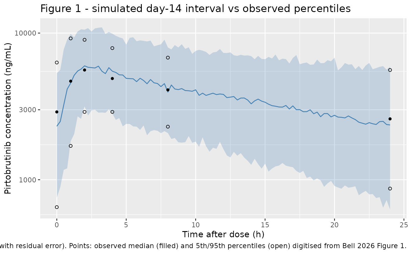
The simulated median and percentiles track the digitised observed percentiles through the dosing interval. The observed band also contains first-dose and lower-dose records (prediction-corrected), so only a qualitative overlay is drawn.

Figure 2: impact of body weight, renal function and albumin

Figure 2A and 2C of Bell 2026 simulate 200 mg once daily for 14 days at the 5th, 50th and 95th percentile of body weight and of serum albumin. The typical profiles (random effects set to zero, other covariates at the reference patient) are shown here.

fig2_levels <- bind_rows(
  tibble(panel = "A: body weight", label = c("WT = 51.8 kg", "WT = 76.6 kg", "WT = 113 kg"),
         WT = c(51.8, 76.6, 113), CRCL = 72.7, ALB = 41.0),
  tibble(panel = "C: serum albumin", label = c("ALB = 31.0 g/L", "ALB = 41.0 g/L", "ALB = 47.8 g/L"),
         WT = 76.6, CRCL = 72.7, ALB = c(31.0, 41.0, 47.8))
) |>
  mutate(id = row_number(), OCC = 1L)

ev_fig2 <- bind_rows(
  fig2_levels |> tidyr::crossing(time = dose_times) |>
    mutate(evid = 1L, amt = 200, cmt = "depot"),
  fig2_levels |> tidyr::crossing(time = seq(0, 24 * 24, by = 0.5)) |>
    mutate(evid = 0L, amt = 0, cmt = "central")
) |>
  arrange(id, time, desc(evid))

sim_fig2 <- rxode2::rxSolve(rxode2::zeroRe(mod), events = ev_fig2,
                            keep = c("panel", "label")) |>
  as.data.frame()
#> Warning: some etas defaulted to non-mu referenced, possible parsing error: etaiov_mtt_1, etaiov_mtt_2, etaiov_mtt_3, etaiov_mtt_4
#> as a work-around try putting the mu-referenced expression on a simple line
#> Warning: some etas defaulted to non-mu referenced, possible parsing error: etaiov_mtt_1, etaiov_mtt_2, etaiov_mtt_3, etaiov_mtt_4
#> as a work-around try putting the mu-referenced expression on a simple line
#> ℹ omega/sigma items treated as zero: 'etalmtt', 'etalcl', 'etaiov_mtt_1', 'etaiov_mtt_2', 'etaiov_mtt_3', 'etaiov_mtt_4'
#> Warning: multi-subject simulation without without 'omega'

ggplot(sim_fig2, aes(time / 24, Cc, colour = label)) +
  geom_line() +
  facet_wrap(~panel, ncol = 1) +
  labs(
    x = "Time (day)", y = "Predicted pirtobrutinib concentration (ng/mL)",
    colour = NULL,
    title = "Figure 2A and 2C - typical profiles at covariate percentiles",
    caption = "Replicates the median lines of Bell 2026 Figure 2A and 2C (200 mg QD for 14 days)."
  )

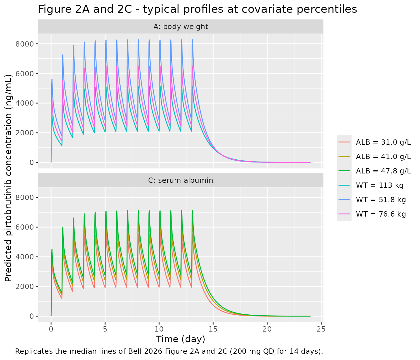
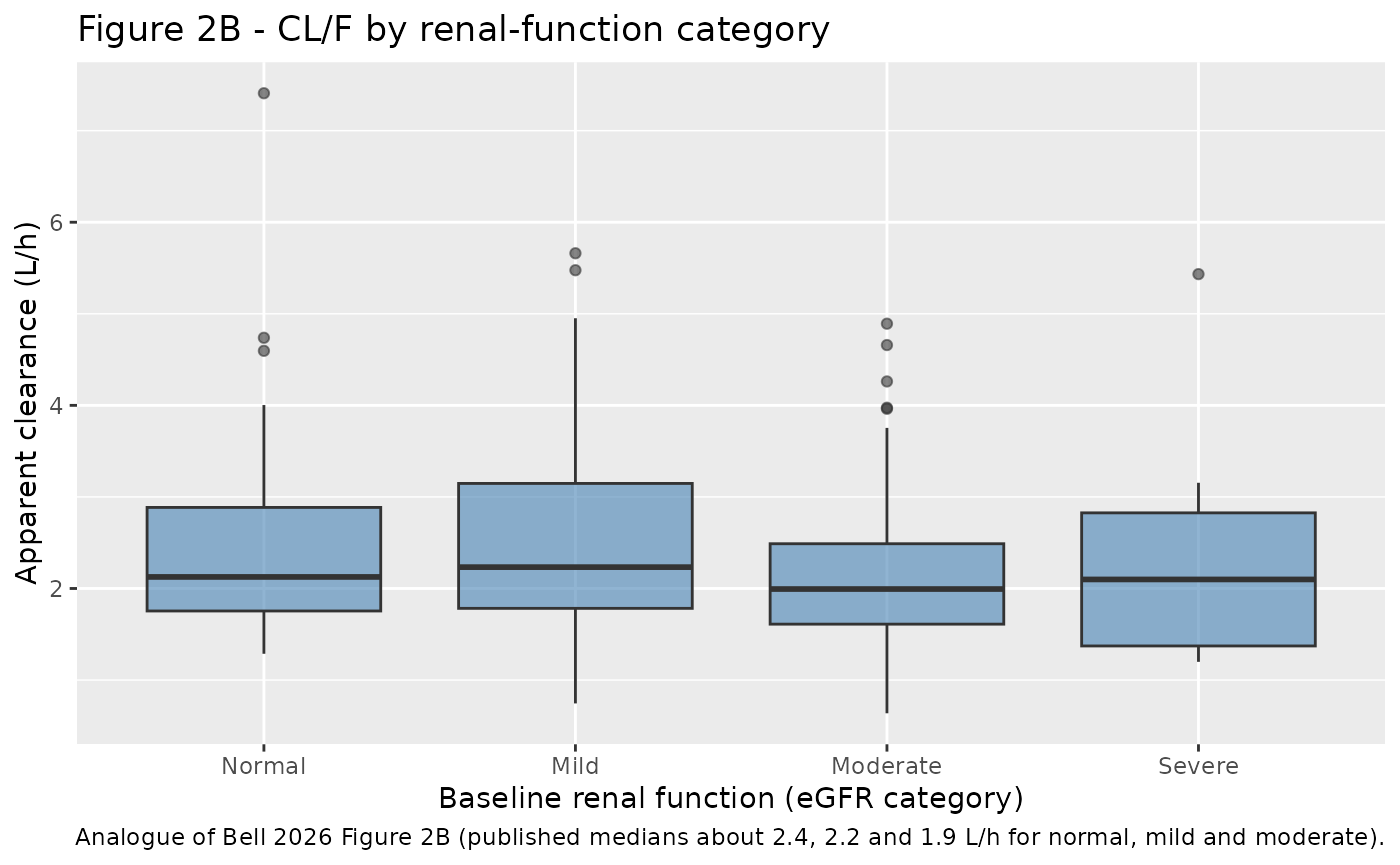
Figure 2B of Bell 2026 shows individual post hoc CL/F by renal-function category. The analogous plot from the virtual cohort (individual CL/F including the interindividual variability):

cl_by_renal <- sim |>
  distinct(id, cl, CRCL) |>
  mutate(
    renal = cut(
      CRCL,
      breaks = c(-Inf, 30, 60, 90, Inf),
      labels = c("Severe", "Moderate", "Mild", "Normal"),
      right = FALSE
    ),
    renal = factor(renal, levels = c("Normal", "Mild", "Moderate", "Severe"))
  )

ggplot(cl_by_renal, aes(renal, cl)) +
  geom_boxplot(fill = "steelblue", alpha = 0.6) +
  labs(
    x = "Baseline renal function (eGFR category)", y = "Apparent clearance (L/h)",
    title = "Figure 2B - CL/F by renal-function category",
    caption = "Analogue of Bell 2026 Figure 2B (published medians about 2.4, 2.2 and 1.9 L/h for normal, mild and moderate)."
  )


cl_by_renal |>
  group_by(renal) |>
  summarise(n = n(), median_cl = round(median(cl), 2), .groups = "drop") |>
  rename("Renal function" = renal, "Median CL/F (L/h)" = median_cl) |>
  knitr::kable()

Renal function	n	Median CL/F (L/h)
Normal	48	2.13
Mild	86	2.23
Moderate	58	1.99
Severe	8	2.10

In the model the typical CL/F differs by only exp(0.00329 * (90 - 45)) = 1.16-fold between an eGFR of 90 and of 45 mL/min/1.73 m^2, against 37.9% CV interindividual variability, so with a few dozen simulated patients per category the category medians can come out in either order. Figure 2B of Bell 2026 makes the same point: the boxes overlap almost completely.

PKNCA validation

Bell 2026 reports, for 200 mg once daily at steady state in phase 2 patients, a geometric mean Cmax of 6460 ng/mL, a mean Cmin of 2260 ng/mL and a mean AUC0-24 of 91,300 ng*h/mL (Results). The day-14 dosing interval of the virtual cohort is analysed with PKNCA (individual predictions, no residual error).

sim_nca <- sim |>
  filter(!is.na(Cc)) |>
  select(id, time, Cc, treatment)

# Guarantee a time-zero row per subject (pre-dose Cc = 0 for oral dosing).
sim_nca <- bind_rows(
  sim_nca,
  sim_nca |> distinct(id, treatment) |> mutate(time = 0, Cc = 0)
) |>
  distinct(id, treatment, time, .keep_all = TRUE) |>
  arrange(id, treatment, time)

conc_obj <- PKNCA::PKNCAconc(sim_nca, Cc ~ time | treatment + id)

dose_df <- events |>
  filter(evid == 1) |>
  select(id, time, amt, treatment)
dose_obj <- PKNCA::PKNCAdose(dose_df, amt ~ time | treatment + id)

intervals <- data.frame(
  start = 13 * 24,
  end = 14 * 24,
  cmax = TRUE,
  cmin = TRUE,
  auclast = TRUE
)

nca_res <- PKNCA::pk.nca(PKNCA::PKNCAdata(conc_obj, dose_obj, intervals = intervals))
nca_long <- as.data.frame(nca_res)

published <- tibble::tribble(
  ~treatment,  ~cmax, ~cmin, ~auclast,
  "200 mg QD", 6460,  2260,  91300
)

cmp <- nlmixr2lib::ncaComparisonTable(
  simulated = nca_long,
  reference = published,
  by = "treatment",
  units = c(cmax = "ng/mL", cmin = "ng/mL", auclast = "ng*h/mL"),
  tolerance_pct = 20
)
knitr::kable(
  cmp,
  caption = "Day-14 steady-state exposure at 200 mg QD: virtual cohort median vs Bell 2026 Results. * differs by >20%."
)

Day-14 steady-state exposure at 200 mg QD: virtual cohort median vs Bell 2026 Results. * differs by >20%.
NCA parameter	treatment	Reference	Simulated	% diff
Cmax (ng/mL)	200 mg QD	6460	6680	+3.4%
Cmin (ng/mL)	200 mg QD	2260	2340	+3.7%
AUClast (ng*h/mL)	200 mg QD	91300	94700	+3.7%


sim_median <- nca_long |>
  filter(PPTESTCD %in% c("cmax", "cmin", "auclast")) |>
  group_by(PPTESTCD) |>
  summarise(value = median(PPORRES), .groups = "drop")
pct_diff <- 100 * (sim_median$value /
  unlist(published[1, sim_median$PPTESTCD]) - 1)
pct_diff
#>  auclast     cmax     cmin 
#> 3.722946 3.446579 3.728667
# A mis-transcribed CL, Vc or dose unit shifts every exposure by tens of
# percent; the cohort medians sit within a few percent of the published values.
stopifnot(all(abs(pct_diff) < 20))

Figure 3: BTK target attainment by dose

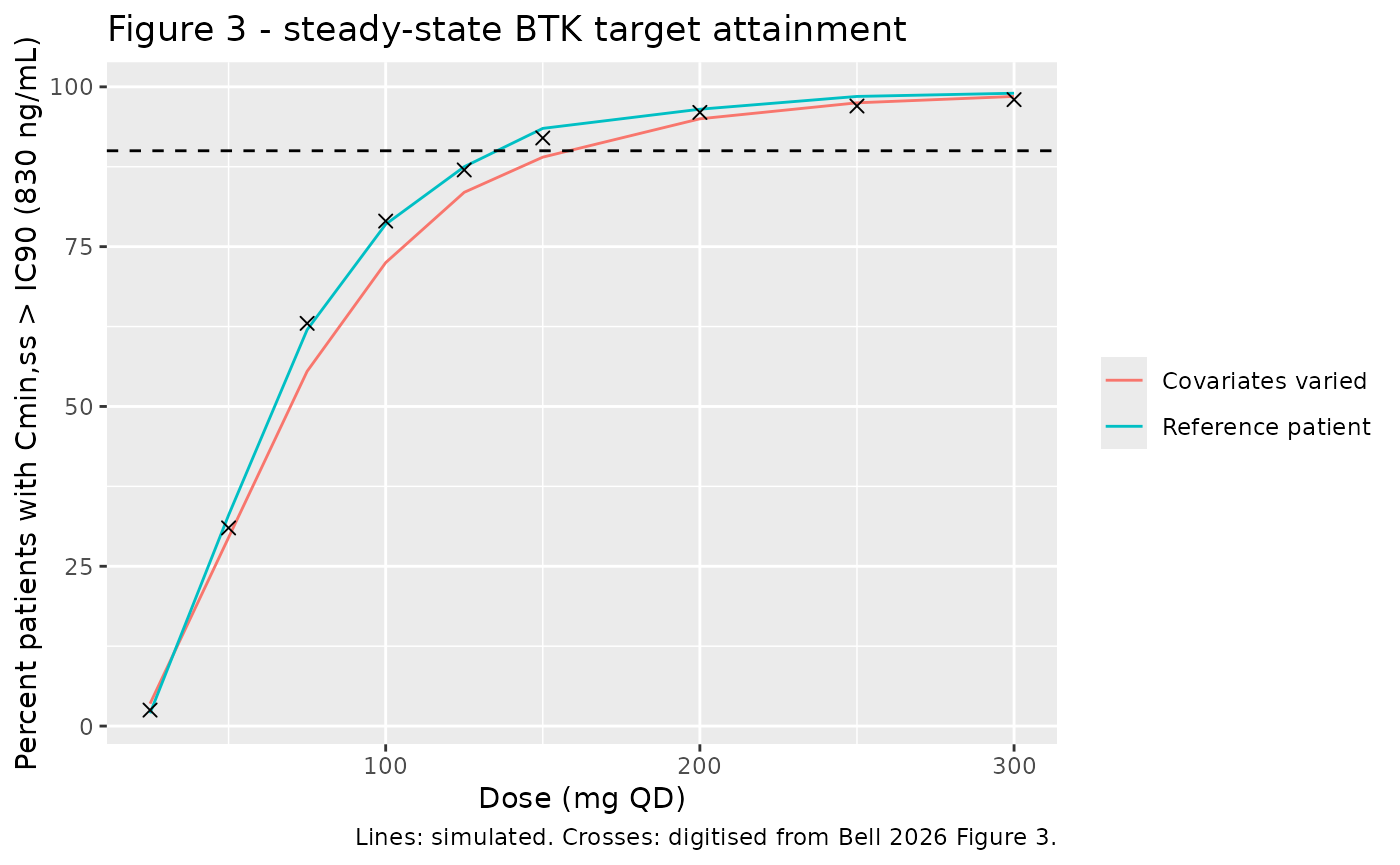
Figure 3 of Bell 2026 plots the percentage of patients whose steady-state Cmin exceeds the protein-binding-adjusted BTK IC90 of 830 ng/mL across 25-300 mg once daily (2000 simulated patients, with interindividual variability). Because the model is linear, Cmin scales exactly with dose, so one steady-state solve per subject at 100 mg gives every dose level. Two 200-subject cohorts are shown: covariates drawn as above, and all covariates at the reference patient.

make_ss_cohort <- function(cov, id_offset) {
  cov |>
    mutate(id = id + id_offset) |>
    tidyr::crossing(tibble(
      time = c(0, 24), evid = c(1L, 0L), amt = c(100, 0),
      ii = c(24, 0), ss = c(1L, 0L), cmt = c("depot", "central")
    ))
}
ss_events <- bind_rows(
  make_ss_cohort(cohort |> mutate(cohort_type = "Covariates varied"), 0L),
  make_ss_cohort(
    cohort |> mutate(WT = 76.6, CRCL = 72.7, ALB = 41.0, cohort_type = "Reference patient"),
    n_sub
  )
) |>
  arrange(id, time, desc(evid))
stopifnot(!anyDuplicated(unique(ss_events[, c("id", "time", "evid")])))

cmin_100 <- rxode2::rxSolve(mod, events = ss_events, keep = "cohort_type") |>
  as.data.frame() |>
  filter(time == 24) |>
  select(id, cohort_type, cmin = Cc)

doses <- c(25, 50, 75, 100, 125, 150, 200, 250, 300)
attain <- tidyr::crossing(cmin_100, dose = doses) |>
  group_by(cohort_type, dose) |>
  summarise(pct = 100 * mean(cmin * dose / 100 > 830), .groups = "drop")

# Digitised by the maintainers from Bell 2026 Figure 3 (band centre); the
# 100 mg and 200 mg values are also stated in the Results text
# ('>= 79%' at >= 100 mg, '96%' at 200 mg).
fig3_pub <- tibble(
  dose = doses,
  pct = c(2.5, 31, 63, 79, 87, 92, 96, 97, 98)
)

ggplot(attain, aes(dose, pct, colour = cohort_type)) +
  geom_line() +
  geom_point(data = fig3_pub, aes(dose, pct), inherit.aes = FALSE, shape = 4, size = 2) +
  geom_hline(yintercept = 90, linetype = "dashed") +
  labs(
    x = "Dose (mg QD)", y = "Percent patients with Cmin,ss > IC90 (830 ng/mL)",
    colour = NULL,
    title = "Figure 3 - steady-state BTK target attainment",
    caption = "Lines: simulated. Crosses: digitised from Bell 2026 Figure 3."
  )


attain |>
  tidyr::pivot_wider(names_from = cohort_type, values_from = pct) |>
  left_join(fig3_pub |> rename(published = pct), by = "dose") |>
  rename("Dose (mg)" = dose, "Published (%)" = published) |>
  knitr::kable(digits = 1)

Dose (mg)	Covariates varied	Reference patient	Published (%)
25	3.5	2.0	2.5
50	29.5	33.0	31.0
75	55.5	62.0	63.0
100	72.5	78.5	79.0
125	83.5	87.5	87.0
150	89.0	93.5	92.0
200	95.0	96.5	96.0
250	97.5	98.5	97.0
300	98.5	99.0	98.0


ref_attain <- attain |> filter(cohort_type == "Reference patient")
# Binomial standard error with 200 subjects is about 1.4 points at 96% and
# 3 points at 79%; the bounds allow for that plus the small systematic gap
# discussed below.
stopifnot(
  abs(ref_attain$pct[ref_attain$dose == 200] - 96) < 6,
  abs(ref_attain$pct[ref_attain$dose == 100] - 79) < 12
)

With covariates fixed at the reference patient the simulated attainment matches the stated 96% at 200 mg and, in a 5000-patient check by the maintainers, sits a few points below the digitised curve between 50 and 125 mg (76.5% vs 79% at 100 mg). Drawing the three covariates independently widens the Cmin distribution slightly and lowers mid-range attainment by a further few points, which suggests Figure 3 was simulated with less covariate spread than this independent-draw cohort (for example the observed, correlated BRUIN covariates or the reference patient).

Assumptions and deviations

Transit-chain convention. Bell 2026 states “4-transit compartments for absorption” and estimates a mean transit time but gives neither the equations nor a diagram. The model uses the Savic parameterisation: the dose enters depot and passes through transit1-transit4 into central, five first-order steps at ktr = 5/MTT, so that MTT is the mean time from dosing to arrival in the central compartment. The alternatives (four steps at ktr = 4/MTT, or five steps at ktr = 4/MTT) give the same AUC and change the typical steady-state Cmax by at most 3% and Tmax by at most 0.4 h, and none of the published secondary results (Figure S2 ratios, Figure 1, the exposure summary) distinguishes them.
Residual error is read as an SD. Table 3 prints “Proportional 0.205” without saying whether it is a variance or a standard deviation. Read as an SD (20.5%), the simulated steady-state 5th percentile at 8 h and 24 h after dose (about 2270 and 830 ng/mL) matches the observed percentiles of Figure 1 (about 2300 and 870 ng/mL); read as a variance (45% CV) the simulated 5th percentiles fall to about 1070 and 380 ng/mL, half the observed values.
Variability scale. Table 3 reports IIV and IOV as CV%; the variances use omega^2 = log(1 + CV^2). The bootstrap percentile intervals do not distinguish this from omega^2 = CV^2, and the difference (0.134 vs 0.144 for CL/F) is small.
Occasions. One MTT inter-occasion variability is reported, but the paper does not define an occasion or the number of occasions. The model carries four occasions, matching the four BRUIN intensive sampling days (Cycle 1 Day 1, Cycle 1 Day 8, Cycle 2 Day 1, Cycle 4 Day 1), with a shared variance. Records with OCC outside 1-4 carry no IOV. The simulations here set OCC = 1 throughout, so the occasion effect acts as additional between-subject variability on MTT. Because the IOV etas enter through occasion indicators, rxode2 warns that they are not mu-referenced; this only affects estimation speed-ups, not simulation.
eGFR centring. The eGFR effect is centred at 74.96 mL/min/1.73 m^2 as printed in the Table 3 footnote, although the Table 2 median is 72 and Figure S2 uses 72.7 for the reference patient. The Figure S2 ratios reproduce exactly with the printed centring.
Virtual cohort. Weight, eGFR and albumin are drawn independently from piecewise-linear interpolations of the published minimum, 5th, 50th and 95th percentile and maximum. Their correlations (albumin enters the MDRD-6 eGFR equation) are not reported.
Covariates screened but not retained (age, sex, race, ethnicity, cancer type, mild hepatic impairment, formulation T1 vs T2) are listed in the model’s covariatesDataExcluded; Bell 2026 reports no coefficients for them.
Digitised values. The Figure 1 observed percentiles and the Figure 3 attainment curve were digitised by the maintainers from the published images and are approximate; the Figure S2 ratios are printed numbers.
No correction notice for Bell 2026 was found in Europe PMC as of 2026-10-08.