Naproxen in arthritic rats (Li 2017)
Source:vignettes/articles/Li_2017_naproxen_rat.Rmd
Li_2017_naproxen_rat.RmdModel and source
- Citation: Li X, DuBois DC, Almon RR, Jusko WJ. Effect of Disease-Related Changes in Plasma Albumin on the Pharmacokinetics of Naproxen in Male and Female Arthritic Rats. Drug Metab Dispos. 2017;45(5):476-483. doi:10.1124/dmd.116.074500.
- Description: Preclinical (rat). Two-compartment population PK model for naproxen (NPX) after intraperitoneal dosing in male and female Lewis rats with collagen-induced arthritis (CIA, a model of rheumatoid arthritis) and in healthy controls (Li 2017). Absorption from the i.p. site is first order with a bioavailability fixed at 0.9 from literature i.v. rat data. The distinguishing feature is that every disposition process operates on UNBOUND drug while both compartments hold TOTAL drug: saturable albumin binding is solved algebraically at each time point, in plasma and again in the tissue interstitial fluid (ISF), and the resulting unbound concentrations drive elimination and distribution. The binding submodel is a Langmuir high-affinity site plus, after the paper’s own Ka2 * Cup << 1 approximation, a linear low-affinity arm; both capacities are proportional to the albumin concentration, so the model reproduces the dose-dependent (nonlinear) PK of naproxen and the hypoalbuminaemia of arthritis from one mechanism. ISF albumin is a fixed fraction of plasma albumin (E/P), higher in arthritis because inflammation raises microvascular permeability. Binding constants were estimated from separate ultrafiltration data and fixed into the PK model; the PK data of all four groups were then fitted jointly by naive pooling in ADAPT 5, so the model carries no between-subject variability.
- Article: Drug Metab Dispos. 2017;45(5):476-483
Population
Naproxen (NPX) was studied in male and female Lewis rats, 5-8 weeks old at purchase and weighing roughly 110-160 g (females) and 170-220 g (males). Collagen-induced arthritis (CIA) was induced with the Chondrex protocol; hind-paw swelling peaked on day 16 in females and day 21 in males, and about 80% of females and 60% of males developed arthritis in one or both hind paws. CIA rats received a single intraperitoneal bolus of sodium naproxen equivalent to 10, 25 or 50 mg/kg NPX on the day of peak disease; age- and sex-matched healthy rats received 50 mg/kg. Three CIA rats and four healthy rats were sampled at each of the 10 post-dose time points (15, 30 and 45 min and 1, 2, 4, 6, 9, 12 and 24 h). Plasma albumin was measured by ELISA in a separate set of animals and plasma protein binding by ultrafiltration over 2-500 ug/mL in pooled plasma from each group.
All protein-binding and PK data were naive-pooled before analysis. The binding profiles were fitted first and the resulting constants were fixed into the PK model, which was then fitted jointly across all four groups in ADAPT 5 by maximum likelihood. Because the analysis was naive-pooled, the published model carries no between-subject variability, so every simulation in this vignette is deterministic and the checks below can be written as exact bounds rather than as quantiles of a random cohort.
The same information is available programmatically via the model’s
population metadata
(readModelDb("Li_2017_naproxen_rat")()$population).
Source trace
The per-parameter origin is recorded as an in-file comment next to
each ini() entry in
inst/modeldb/specificDrugs/Li_2017_naproxen_rat.R. The
table below collects them in one place for review.
| Equation / parameter | Value | Source location |
|---|---|---|
Two-class Langmuir plasma binding,
Cbp = n1*Pt*Ka1*Cup/(1+Ka1*Cup) + n2*Pt*Ka2*Cup/(1+Ka2*Cup)
|
n/a | Equation 1, p. 477 |
Cbp = Cp - Cup |
n/a | Equation 2, p. 477 |
Quadratic in Cup after the stated
Ka2*Cup << 1 approximation |
n/a | Equation 3, p. 477 |
Positive root
Cup = (-b + sqrt(b^2 + 4*a*Cp))/(2*a)
|
n/a | Equation 4, p. 477 |
Tissue binding: the same equation with Pt multiplied by
E/P
|
n/a | Methods, paragraph after equation 4 |
d/dt(depot) = -ka*depot,
Aa(0) = dose*F
|
n/a | Equation 5, p. 477 |
Vp*dCp/dt = ka*Aa + CLd*(Cut - Cup) - CL*Cup |
n/a | Equation 6, p. 477 |
Vt*dCt/dt = CLd*(Cup - Cut) |
n/a | Equation 7, p. 477 |
Variance model Vi = (s1 + s2*Yi)^2
|
s1, s2 not reported | Equation 8, p. 479 |
lka |
0.814 1/h | Table 4 |
lcl_cia / lcl_healthy
|
1370 / 1879 mL/h/kg | Table 4 |
lq_cia / lq_healthy
|
647.2 / 1371 mL/h/kg | Table 4 |
lvp_cia / lvp_healthy
|
140.7 / 114.7 mL/kg | Table 4 |
lvc (fixed) |
32.36 mL/kg | Table 4, footnote a (rat plasma volume, Shah and Betts 2012) |
lfdepot (fixed) |
0.9 | Methods, paragraph after equation 7 (Lauroba 1986) |
kaff_cf / kaff_hf / kaff_cm /
kaff_hm (fixed) |
0.28 / 0.25 / 0.26 / 0.26 L/umol | Table 1, Ka1 row |
kaff2_cf / kaff2_hf /
kaff2_cm / kaff2_hm (fixed) |
0.0041 / 0.0043 / 0.0056 / 0.0054 L/umol | Table 1, Ka2 row |
n1 = 1, n2 = 4 (literals in
model()) |
1, 4 | Table 1, both marked Fixed |
ALB covariate values |
347 / 550 / 282 / 422 umol/L | Table 1, Pt row; Fig. 2 |
f_alb_isf_cia / f_alb_isf_healthy
(fixed) |
0.9 / 0.5 | Discussion, “different E/P values were assigned” paragraph |
| Naproxen molecular weight 230.26 g/mol | literal in model()
|
corroborated by the LC-MS/MS transition m/z 229.2 for [M-H]-, Methods |
| Albumin molecular weight 66500 g/mol | literal in model()
|
inst/references/covariate-columns.md, ALB
entry |
Virtual cohort
The original animal-level data are not publicly available. Because the published model has no between-subject variability, one representative animal per study arm reproduces the published typical-value predictions exactly; there is nothing for a larger cohort to average over. The eight arms below are the six CIA arms (two sexes at 10, 25 and 50 mg/kg) and the two healthy arms (two sexes at 50 mg/kg).
Albumin is carried as the canonical ALB column in SI
g/L, converted from the umol/L of Table 1 with albumin molecular weight
66500 g/mol.
arms <- tidyr::expand_grid(
  tibble::tibble(
    group   = c("CIA female", "Healthy female", "CIA male", "Healthy male"),
    SEXF    = c(1, 1, 0, 0),
    DIS_CIA = c(1, 0, 1, 0),
    # Table 1 "Pt (uM)": measured plasma albumin, marked Fixed.
    Pt_uM   = c(347, 550, 282, 422)
  ),
  dose_mgkg = c(10, 25, 50)
) |>
  # Only the CIA rats received the 10 and 25 mg/kg doses; the healthy rats
  # were studied at 50 mg/kg only (Methods, "Pharmacokinetics of NPX").
  dplyr::filter(DIS_CIA == 1 | dose_mgkg == 50) |>
  dplyr::mutate(
    id        = dplyr::row_number(),
    ALB       = Pt_uM * 66500 / 1e6,
    treatment = paste0(group, ", ", dose_mgkg, " mg/kg")
  )

knitr::kable(
  arms |>
    dplyr::select(treatment, SEXF, DIS_CIA, Pt_uM, ALB, dose_mgkg) |>
    dplyr::mutate(ALB = round(ALB, 1)) |>
    dplyr::rename(
      "Arm"                 = treatment,
      "SEXF"                = SEXF,
      "DIS_CIA"             = DIS_CIA,
      "Albumin (umol/L)"    = Pt_uM,
      "ALB (g/L)"           = ALB,
      "NPX dose (mg/kg)"    = dose_mgkg
    ),
  caption = "Study arms of Li 2017 and the covariate values each carries."
)| Arm | SEXF | DIS_CIA | Albumin (umol/L) | ALB (g/L) | NPX dose (mg/kg) |
|---|---|---|---|---|---|
| CIA female, 10 mg/kg | 1 | 1 | 347 | 23.1 | 10 |
| CIA female, 25 mg/kg | 1 | 1 | 347 | 23.1 | 25 |
| CIA female, 50 mg/kg | 1 | 1 | 347 | 23.1 | 50 |
| Healthy female, 50 mg/kg | 1 | 0 | 550 | 36.6 | 50 |
| CIA male, 10 mg/kg | 0 | 1 | 282 | 18.8 | 10 |
| CIA male, 25 mg/kg | 0 | 1 | 282 | 18.8 | 25 |
| CIA male, 50 mg/kg | 0 | 1 | 282 | 18.8 | 50 |
| Healthy male, 50 mg/kg | 0 | 0 | 422 | 28.1 | 50 |
# Dense grid for the profile figures and the unbound-exposure identity; the
# paper's own sampling times are used separately for the NCA comparison so
# that the simulated and published NCA see the same design.
dense_times <- sort(unique(c(seq(0, 24, by = 0.02), seq(24, 240, by = 0.5))))

events <-
  dplyr::bind_rows(
    # Dose records: amt in ug/kg (dose_mgkg * 1000).
    arms |>
      dplyr::transmute(
        id, treatment, group, dose_mgkg, SEXF, DIS_CIA, ALB,
        time = 0, amt = dose_mgkg * 1000, evid = 1L, cmt = "depot"
      ),
    # Observation records on the central ODE state; rxode2 returns the
    # algebraic observables Cc and Cu as columns at these rows.
    arms |>
      dplyr::select(id, treatment, group, dose_mgkg, SEXF, DIS_CIA, ALB) |>
      tidyr::expand_grid(time = dense_times) |>
      dplyr::mutate(amt = NA_real_, evid = 0L, cmt = "central")
  ) |>
  dplyr::arrange(id, time, dplyr::desc(evid))

stopifnot(!anyDuplicated(events[events$evid == 0L, c("id", "time")]))
Simulation
mod <- readModelDb("Li_2017_naproxen_rat")

sim <- rxode2::rxSolve(
  mod,
  events = events,
  keep   = c("treatment", "group", "dose_mgkg")
) |>
  as.data.frame() |>
  dplyr::filter(!is.na(Cc))
#> Warning: multi-subject simulation without without 'omega'
Cc is the total plasma naproxen concentration that the
LC-MS/MS assay measured and that the variance model of equation 8
applies to; Cu is the unbound plasma concentration that
drives every disposition process.
Replicate published figures
# Replicates Figure 5 of Li 2017: total (upper) and model-predicted unbound
# (lower) plasma NPX in CIA rats at 10, 25 and 50 mg/kg, by sex.
sim |>
  dplyr::filter(group %in% c("CIA female", "CIA male"), time <= 24) |>
  tidyr::pivot_longer(c(Cc, Cu), names_to = "analyte", values_to = "conc") |>
  dplyr::mutate(
    analyte = factor(
      analyte,
      levels = c("Cc", "Cu"),
      labels = c("Total NPX", "Unbound NPX")
    ),
    dose = factor(paste(dose_mgkg, "mg/kg"), levels = paste(c(10, 25, 50), "mg/kg"))
  ) |>
  ggplot(aes(time, conc, colour = dose, linetype = dose)) +
  geom_line() +
  facet_grid(analyte ~ group, scales = "free_y") +
  scale_y_log10() +
  labs(
    x = "Time (h)", y = "Plasma NPX concentration (ug/mL)",
    colour = NULL, linetype = NULL,
    title = "Figure 5 - dose-ranging profiles in CIA rats",
    caption = "Replicates Figure 5 of Li 2017."
  ) +
  theme(legend.position = "bottom")
#> Warning in scale_y_log10(): log-10 transformation introduced infinite values.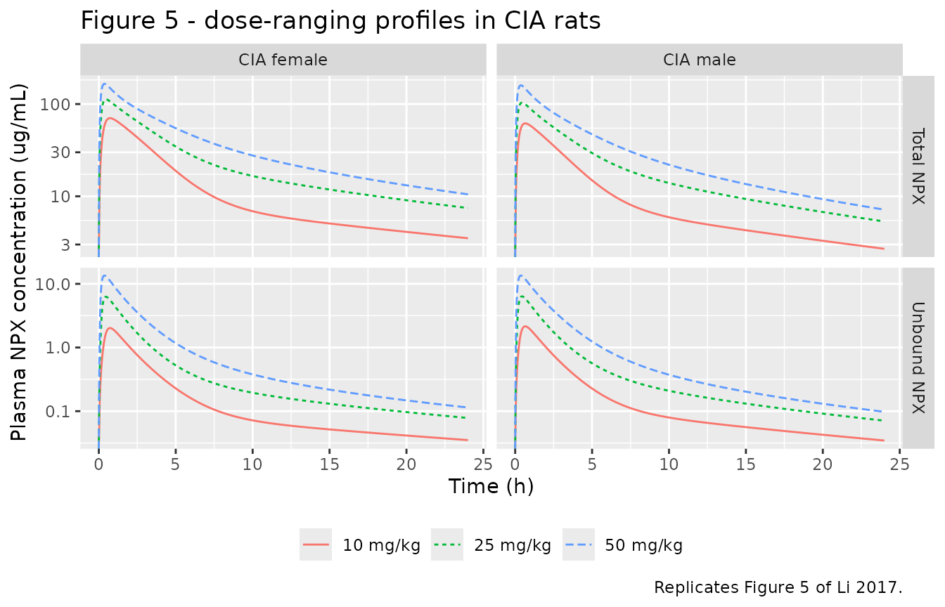
# Replicates Figure 7 of Li 2017: simulated unbound plasma NPX for the four
# 50 mg/kg groups; arthritic rats sit above healthy rats in both sexes.
sim |>
  dplyr::filter(dose_mgkg == 50, time <= 24) |>
  ggplot(aes(time, Cu, colour = group, linetype = group)) +
  geom_line() +
  scale_y_log10() +
  labs(
    x = "Time (h)", y = "Unbound plasma NPX (ug/mL)",
    colour = NULL, linetype = NULL,
    title = "Figure 7 - unbound profiles at 50 mg/kg",
    caption = "Replicates Figure 7 of Li 2017."
  ) +
  theme(legend.position = "bottom")
#> Warning in scale_y_log10(): log-10 transformation introduced infinite values.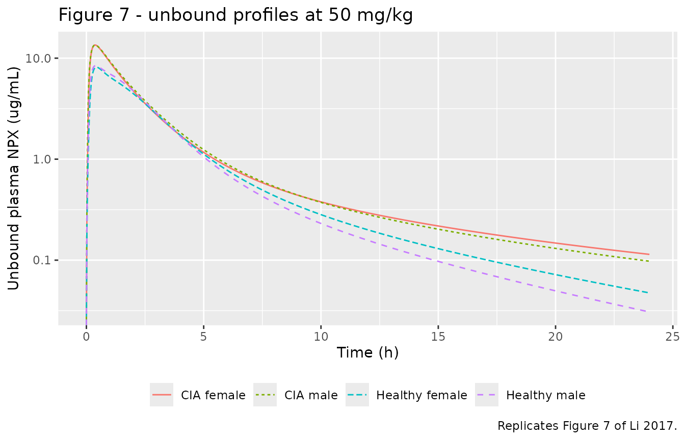
The binding submodel can also be exercised on its own, without solving the PK model, by evaluating the positive root of equation 3 over the range of total concentrations used in the ultrafiltration experiment.
# Replicates Figure 4 (bound vs unbound) and the Figure 3 insets (unbound
# fraction vs total concentration) of Li 2017.
binding_root <- function(Ctot_ugmL, Pt_uM, Ka1, Ka2, n1 = 1, n2 = 4) {
  Ctot <- Ctot_ugmL * 1000 / 230.26
  a <- Ka1 * (1 + n2 * Pt_uM * Ka2)
  b <- n1 * Pt_uM * Ka1 + n2 * Pt_uM * Ka2 - Ctot * Ka1 + 1
  ((-b + sqrt(b * b + 4 * a * Ctot)) / (2 * a)) * 230.26 / 1000
}

binding_constants <- tibble::tibble(
  group = c("CIA female", "Healthy female", "CIA male", "Healthy male"),
  Pt_uM = c(347, 550, 282, 422),
  Ka1   = c(0.28, 0.25, 0.26, 0.26),
  Ka2   = c(0.0041, 0.0043, 0.0056, 0.0054)
)

binding <- binding_constants |>
  tidyr::expand_grid(Ctot = c(2, 5, 10, 20, 50, 100, 200, 500)) |>
  dplyr::mutate(
    Cu     = binding_root(Ctot, Pt_uM, Ka1, Ka2),
    Cbound = Ctot - Cu,
    fu     = Cu / Ctot
  )

ggplot(binding, aes(Cu, Cbound, colour = group)) +
  geom_line() +
  geom_point() +
  labs(
    x = "Unbound NPX (ug/mL)", y = "Bound NPX (ug/mL)", colour = NULL,
    title = "Figure 4 - bound versus unbound naproxen",
    caption = "Replicates Figure 4 of Li 2017 (equation 1 under the stated Ka2*Cup << 1 approximation)."
  ) +
  theme(legend.position = "bottom")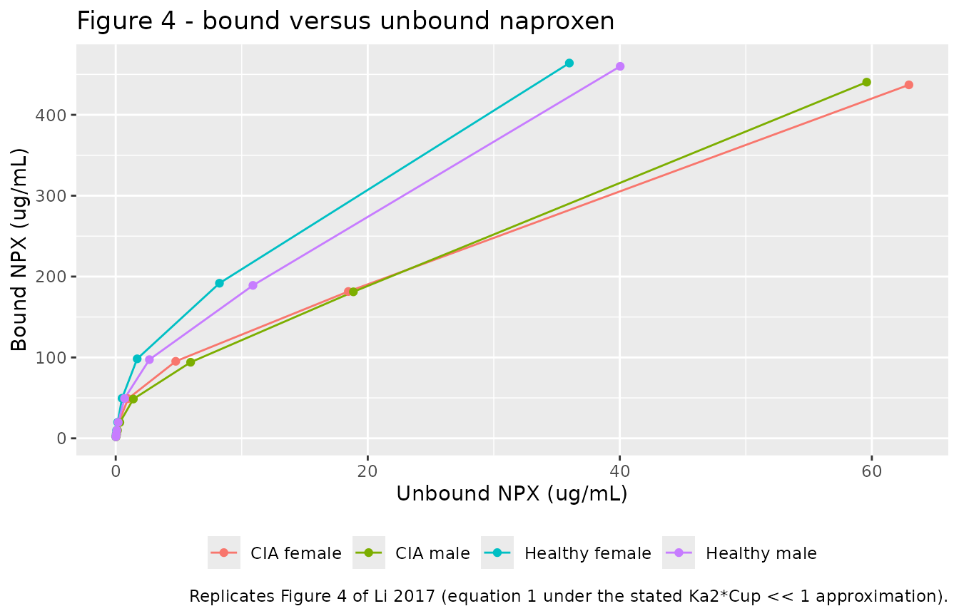
ggplot(binding, aes(Ctot, 100 * fu, colour = group)) +
  geom_line() +
  geom_point() +
  scale_x_log10() +
  labs(
    x = "Total NPX (ug/mL)", y = "Unbound fraction (%)", colour = NULL,
    title = "Figure 3 inset - unbound fraction versus total concentration",
    caption = "Replicates the embedded fu-versus-Ct panels of Figure 3 of Li 2017."
  ) +
  theme(legend.position = "bottom")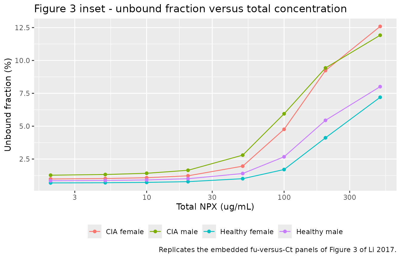
# Results, "Protein Binding of NPX": ">93%" bound at normal therapeutic
# concentrations, with a significant decrease above 50 ug/mL total in CIA rats
# and above 100 ug/mL in healthy rats. The binding submodel must reproduce both
# the level and the ordering (CIA rats less bound than healthy rats of the same
# sex, because CIA rats have less albumin).
pb <- binding |>
  dplyr::select(group, Ctot, fu) |>
  tidyr::pivot_wider(names_from = group, values_from = fu)

stopifnot(
  # >93% bound (fu < 7%) at and below the 20 ug/mL therapeutic range.
  all(binding$fu[binding$Ctot <= 20] < 0.07),
  # Saturation is real: the unbound fraction rises steeply above 50 ug/mL.
  all(binding$fu[binding$Ctot == 500] > 3 * binding$fu[binding$Ctot == 2]),
  # Arthritis lowers albumin and therefore lowers binding, within each sex.
  all(pb[["CIA female"]] > pb[["Healthy female"]]),
  all(pb[["CIA male"]] > pb[["Healthy male"]])
)
Structural checks
Every disposition process in this model operates on unbound drug, so
the unbound exposure has a closed form that is completely independent of
the binding submodel: at steady state of the mass balance,
AUC_unbound(0-Inf) = dose * F / CL. That identity is the
primary structural gate here – a mis-transcribed clearance, dose,
bioavailability or unit would break it immediately, and because the
model is deterministic the agreement is numerical rather than
statistical.
trapz <- function(t, y) sum(diff(t) * (utils::head(y, -1) + utils::tail(y, -1)) / 2)

auc_check <- sim |>
  dplyr::group_by(treatment, group, dose_mgkg) |>
  dplyr::summarise(auc_u = trapz(time, Cu), .groups = "drop") |>
  dplyr::mutate(
    arthritic   = grepl("^CIA", group),
    cl_pub      = ifelse(arthritic, 1370, 1879),   # Table 4, mL/h/kg
    auc_u_exact = dose_mgkg * 1000 * 0.9 / cl_pub, # dose (ug/kg) * F / CL
    pct_diff    = 100 * (auc_u - auc_u_exact) / auc_u_exact
  )

knitr::kable(
  auc_check |>
    dplyr::select(treatment, auc_u, auc_u_exact, pct_diff) |>
    dplyr::rename(
      "Arm"                              = treatment,
      "Simulated AUC unbound (ug*h/mL)"  = auc_u,
      "dose * F / CL (ug*h/mL)"          = auc_u_exact,
      "Difference (%)"                   = pct_diff
    ),
  digits = 3,
  caption = "Unbound exposure against its closed form. The integration runs to 240 h, so the only residual is truncation and quadrature error."
)| Arm | Simulated AUC unbound (ug*h/mL) | dose * F / CL (ug*h/mL) | Difference (%) |
|---|---|---|---|
| CIA female, 10 mg/kg | 6.569 | 6.569 | -0.013 |
| CIA female, 25 mg/kg | 16.422 | 16.423 | -0.009 |
| CIA female, 50 mg/kg | 32.845 | 32.847 | -0.006 |
| CIA male, 10 mg/kg | 6.569 | 6.569 | -0.002 |
| CIA male, 25 mg/kg | 16.423 | 16.423 | -0.002 |
| CIA male, 50 mg/kg | 32.846 | 32.847 | -0.002 |
| Healthy female, 50 mg/kg | 23.949 | 23.949 | -0.001 |
| Healthy male, 50 mg/kg | 23.949 | 23.949 | -0.001 |
The paper prints four unbound anchors for the 50 mg/kg arms in the Results (“Pharmacokinetics of NPX”): peak unbound concentrations of 13.52 vs 8.14 ug/mL for CIA versus healthy females and 13.51 vs 8.43 ug/mL for males, and unbound AUCs of 32.76 vs 23.94 and 32.82 vs 23.95 ug*h/mL. These exercise the binding submodel, which the closed form above does not.
published_unbound <- tibble::tribble(
  ~group,           ~cmax_u_pub, ~auc_u_pub,
  "CIA female",     13.52,       32.76,
  "Healthy female",  8.14,       23.94,
  "CIA male",       13.51,       32.82,
  "Healthy male",    8.43,       23.95
)

anchors <- sim |>
  dplyr::filter(dose_mgkg == 50) |>
  dplyr::group_by(group) |>
  dplyr::summarise(cmax_u = max(Cu), auc_u = trapz(time, Cu), .groups = "drop") |>
  dplyr::left_join(published_unbound, by = "group") |>
  dplyr::mutate(
    pct_cmax = 100 * (cmax_u - cmax_u_pub) / cmax_u_pub,
    pct_auc  = 100 * (auc_u - auc_u_pub) / auc_u_pub
  )

knitr::kable(
  anchors |>
    dplyr::rename(
      "Group"                        = group,
      "Simulated Cmax unbound"       = cmax_u,
      "Published Cmax unbound"       = cmax_u_pub,
      "Cmax difference (%)"          = pct_cmax,
      "Simulated AUC unbound"        = auc_u,
      "Published AUC unbound"        = auc_u_pub,
      "AUC difference (%)"           = pct_auc
    ),
  digits = 3,
  caption = "Unbound Cmax (ug/mL) and AUC (ug*h/mL) at 50 mg/kg against the values printed in the Results of Li 2017."
)| Group | Simulated Cmax unbound | Simulated AUC unbound | Published Cmax unbound | Published AUC unbound | Cmax difference (%) | AUC difference (%) |
|---|---|---|---|---|---|---|
| CIA female | 13.489 | 32.845 | 13.52 | 32.76 | -0.228 | 0.259 |
| CIA male | 13.477 | 32.846 | 13.51 | 32.82 | -0.242 | 0.080 |
| Healthy female | 8.142 | 23.949 | 8.14 | 23.94 | 0.022 | 0.037 |
| Healthy male | 8.437 | 23.949 | 8.43 | 23.95 | 0.079 | -0.006 |
stopifnot(
  # Peak unbound concentration depends on the whole binding submodel, the
  # absorption rate and the distribution clearance, so 1% agreement on all
  # four arms is a strong joint check on the transcription.
  max(abs(anchors$pct_cmax)) < 1,
  # The published unbound AUCs are the closed form rounded to four figures.
  max(abs(anchors$pct_auc)) < 1
)
The paper’s central claim is that saturable albumin binding, and nothing else, produces the dose-dependent PK of total naproxen: the Results report that the dose-normalised AUC of total drug “decreased nearly 2-fold over the 5-fold range of doses” in CIA rats, while “the PK parameters based on free drug were independent of dose” (Discussion). Both halves are checkable.
nonlin <- sim |>
  dplyr::filter(group %in% c("CIA female", "CIA male")) |>
  dplyr::group_by(group, dose_mgkg) |>
  dplyr::summarise(
    auc_tot = trapz(time, Cc),
    auc_u   = trapz(time, Cu),
    .groups = "drop"
  ) |>
  dplyr::mutate(dn_auc_tot = auc_tot / dose_mgkg, dn_auc_u = auc_u / dose_mgkg)

ratio_tot <- nonlin |>
  dplyr::select(group, dose_mgkg, dn_auc_tot) |>
  tidyr::pivot_wider(names_from = dose_mgkg, values_from = dn_auc_tot, names_prefix = "d") |>
  dplyr::mutate(ratio = d10 / d50)

ratio_u <- nonlin |>
  dplyr::select(group, dose_mgkg, dn_auc_u) |>
  tidyr::pivot_wider(names_from = dose_mgkg, values_from = dn_auc_u, names_prefix = "d") |>
  dplyr::mutate(ratio = d10 / d50)

knitr::kable(
  dplyr::bind_rows(
    ratio_tot |> dplyr::mutate(analyte = "Total NPX"),
    ratio_u |> dplyr::mutate(analyte = "Unbound NPX")
  ) |>
    dplyr::select(analyte, group, ratio) |>
    dplyr::rename(
      "Analyte"                                   = analyte,
      "Group"                                     = group,
      "Dose-normalised AUC, 10 mg/kg / 50 mg/kg"  = ratio
    ),
  digits = 3,
  caption = "Nonlinearity of total naproxen exposure and its absence for unbound naproxen."
)| Analyte | Group | Dose-normalised AUC, 10 mg/kg / 50 mg/kg |
|---|---|---|
| Total NPX | CIA female | 1.866 |
| Total NPX | CIA male | 1.845 |
| Unbound NPX | CIA female | 1.000 |
| Unbound NPX | CIA male | 1.000 |
stopifnot(
  # "decreased nearly 2-fold over the 5-fold range of doses" (Results).
  all(ratio_tot$ratio > 1.5), all(ratio_tot$ratio < 2.5),
  # "The PK parameters based on free drug were independent of dose"
  # (Discussion) -- unbound exposure is exactly dose proportional.
  max(abs(ratio_u$ratio - 1)) < 0.01
)
PKNCA validation
The published NCA was run on the observed total-drug concentrations at the study’s own sampling times, so the simulated profiles are re-sampled onto that design before the NCA rather than using the dense grid.
# Li 2017 Methods, "Pharmacokinetics of NPX": 15, 30 and 45 minutes and 1, 2,
# 4, 6, 9, 12 and 24 hours post dose.
nca_times <- c(0.25, 0.5, 0.75, 1, 2, 4, 6, 9, 12, 24)

sim_nca <- sim |>
  dplyr::filter(!is.na(Cc), time %in% nca_times) |>
  dplyr::select(id, time, Cc, treatment)

# Extravascular dosing, so the pre-dose concentration is zero; PKNCA needs the
# time-zero row to anchor AUC0-*.
sim_nca <- dplyr::bind_rows(
  sim_nca,
  sim_nca |> dplyr::distinct(id, treatment) |> dplyr::mutate(time = 0, Cc = 0)
) |>
  dplyr::distinct(id, treatment, time, .keep_all = TRUE) |>
  dplyr::arrange(id, treatment, time)

conc_obj <- PKNCA::PKNCAconc(sim_nca, Cc ~ time | treatment + id)

dose_df <- events |>
  dplyr::filter(evid == 1L) |>
  dplyr::select(id, time, amt, treatment)

dose_obj <- PKNCA::PKNCAdose(dose_df, amt ~ time | treatment + id)

intervals <- data.frame(
  start       = 0,
  end         = Inf,
  cmax        = TRUE,
  tmax        = TRUE,
  auclast     = TRUE,
  aucinf.obs  = TRUE,
  aucpext.obs = TRUE,
  half.life   = TRUE,
  cl.obs      = TRUE,
  vz.obs      = TRUE
)

nca_res <- PKNCA::pk.nca(PKNCA::PKNCAdata(conc_obj, dose_obj, intervals = intervals))
Comparison against published NCA
Li 2017 Table 2 reports dose-normalised AUC, CL/F, V/F and terminal half-life for the three CIA dose groups in each sex, and Table 3 repeats the 50 mg/kg rows alongside the healthy groups. The AUC values below are recovered from Table 2’s dose-normalised AUC by multiplying by the dose, except for the four 50 mg/kg arms, which Table 3 prints directly.
published <- tibble::tribble(
  ~treatment,                    ~aucinf.obs, ~cl.obs, ~vz.obs, ~half.life,
  "CIA female, 10 mg/kg",         338.4,      29.98,   133.8,   3.13,
  "CIA female, 25 mg/kg",         636.0,      39.34,   157.0,   2.76,
  "CIA female, 50 mg/kg",         936.0,      53.43,   287.1,   3.74,
  "CIA male, 10 mg/kg",           270.9,      36.98,   135.1,   2.54,
  "CIA male, 25 mg/kg",           606.5,      41.31,   137.9,   2.32,
  "CIA male, 50 mg/kg",           809.8,      61.99,   229.3,   2.55,
  "Healthy female, 50 mg/kg",    1203.4,      41.89,   188.6,   3.13,
  "Healthy male, 50 mg/kg",      1054.5,      47.76,   169.7,   2.46
)

cmp <- nlmixr2lib::ncaComparisonTable(
  simulated = nca_res,
  reference = published,
  by        = "treatment",
  # cmax / tmax / auclast / aucpext.obs are computed above for the diagnostics
  # below but have no published counterpart, so they are excluded here.
  params    = c("aucinf.obs", "cl.obs", "vz.obs", "half.life"),
  units     = c(
    aucinf.obs = "ug*h/mL", cl.obs = "mL/h/kg",
    vz.obs = "mL/kg", half.life = "h"
  ),
  tolerance_pct = 20
)

knitr::kable(
  cmp,
  caption = "Simulated versus published NCA on total naproxen. * differs from the reference by more than 20%.",
  align   = c("l", "l", "r", "r", "r")
)| NCA parameter | treatment | Reference | Simulated | % diff |
|---|---|---|---|---|
| AUC0-∞ (obs) (ug*h/mL) | CIA female, 10 mg/kg | 338 | 400 | +18.3% |
| AUC0-∞ (obs) (ug*h/mL) | CIA female, 25 mg/kg | 636 | 724 | +13.9% |
| AUC0-∞ (obs) (ug*h/mL) | CIA female, 50 mg/kg | 936 | 1040 | +11.1% |
| AUC0-∞ (obs) (ug*h/mL) | CIA male, 10 mg/kg | 271 | 321 | +18.5% |
| AUC0-∞ (obs) (ug*h/mL) | CIA male, 25 mg/kg | 606 | 582 | -4.1% |
| AUC0-∞ (obs) (ug*h/mL) | CIA male, 50 mg/kg | 810 | 846 | +4.5% |
| AUC0-∞ (obs) (ug*h/mL) | Healthy female, 50 mg/kg | 1200 | 1190 | -1.0% |
| AUC0-∞ (obs) (ug*h/mL) | Healthy male, 50 mg/kg | 1050 | 905 | -14.1% |
| t½ (h) | CIA female, 10 mg/kg | 3.13 | 13.9 | +343.9%* |
| t½ (h) | CIA female, 25 mg/kg | 2.76 | 12 | +333.0%* |
| t½ (h) | CIA female, 50 mg/kg | 3.74 | 9.91 | +165.1%* |
| t½ (h) | CIA male, 10 mg/kg | 2.54 | 12.1 | +374.5%* |
| t½ (h) | CIA male, 25 mg/kg | 2.32 | 10 | +331.2%* |
| t½ (h) | CIA male, 50 mg/kg | 2.55 | 8.57 | +236.2%* |
| t½ (h) | Healthy female, 50 mg/kg | 3.13 | 6.09 | +94.4%* |
| t½ (h) | Healthy male, 50 mg/kg | 2.46 | 5.25 | +113.2%* |
| CL/F (mL/h/kg) | CIA female, 10 mg/kg | 30 | 25 | -16.7% |
| CL/F (mL/h/kg) | CIA female, 25 mg/kg | 39.3 | 34.5 | -12.3% |
| CL/F (mL/h/kg) | CIA female, 50 mg/kg | 53.4 | 48.1 | -10.0% |
| CL/F (mL/h/kg) | CIA male, 10 mg/kg | 37 | 31.1 | -15.8% |
| CL/F (mL/h/kg) | CIA male, 25 mg/kg | 41.3 | 43 | +4.0% |
| CL/F (mL/h/kg) | CIA male, 50 mg/kg | 62 | 59.1 | -4.6% |
| CL/F (mL/h/kg) | Healthy female, 50 mg/kg | 41.9 | 42 | +0.2% |
| CL/F (mL/h/kg) | Healthy male, 50 mg/kg | 47.8 | 55.2 | +15.6% |
| Vz/F (mL/kg) | CIA female, 10 mg/kg | 134 | 501 | +274.1%* |
| Vz/F (mL/kg) | CIA female, 25 mg/kg | 157 | 595 | +279.0%* |
| Vz/F (mL/kg) | CIA female, 50 mg/kg | 287 | 688 | +139.5%* |
| Vz/F (mL/kg) | CIA male, 10 mg/kg | 135 | 542 | +300.9%* |
| Vz/F (mL/kg) | CIA male, 25 mg/kg | 138 | 620 | +349.8%* |
| Vz/F (mL/kg) | CIA male, 50 mg/kg | 229 | 731 | +218.8%* |
| Vz/F (mL/kg) | Healthy female, 50 mg/kg | 189 | 369 | +95.4%* |
| Vz/F (mL/kg) | Healthy male, 50 mg/kg | 170 | 418 | +146.3%* |
Read this table by parameter, not row by row.
Exposure and clearance agree. Every
AUC0-Inf and CL/F row is inside the 20% band,
and the dose-dependence the paper reports is reproduced in the right
direction and roughly the right size: simulated CL/F and
Vz/F both rise with dose in the CIA rats, which is the NCA
signature of saturating albumin binding rather than of a saturating
elimination pathway.
Terminal half-life, and therefore Vz/F, does not
agree, and the gap is a property of the published model rather than of
the transcription. Two things have to be separated here. The
unbound anchors above are model outputs and reproduce to within
1%, so the parameters are transcribed correctly. Tables 2 and 3, by
contrast, are non-compartmental summaries of the observed data,
and the model’s late-time decline is markedly slower than theirs.
The reason is structural. At low concentrations the binding is effectively linear and naproxen is about 99% bound, so the tissue interstitium acts as a deep reservoir of drug that is released only as fast as the small unbound fraction allows. The chunk below reads the model’s own local half-life off the simulated curve over the study’s sampling window and, separately, derives the true terminal half-life the model implies once binding has linearised.
local_half_life <- function(d, from, to) {
  d <- d[d$time >= from & d$time <= to, ]
  log(2) / -stats::coef(stats::lm(log(Cc) ~ time, data = d))[[2]]
}

# Linear-regime (low-concentration) micro-constants. As Cu -> 0 the binding
# model collapses to Ctot = Cu * (1 + n1*Pt*Ka1 + n2*Pt*Ka2), so the unbound
# drug behaves as a two-compartment linear system with inflated volumes.
terminal_from_micro <- function(Pt_uM, Ka1, Ka2, ep, vc, vp, cl, q, n1 = 1, n2 = 4) {
  ratio_p <- 1 + n1 * Pt_uM * Ka1 + n2 * Pt_uM * Ka2
  ratio_t <- 1 + n1 * (ep * Pt_uM) * Ka1 + n2 * (ep * Pt_uM) * Ka2
  vc_u <- vc * ratio_p
  vt_u <- vp * ratio_t
  kel <- cl / vc_u
  k12 <- q / vc_u
  k21 <- q / vt_u
  s <- kel + k12 + k21
  log(2) / ((s - sqrt(s * s - 4 * kel * k21)) / 2)
}

published_thalf <- tibble::tibble(
  group            = c("CIA female", "Healthy female", "CIA male", "Healthy male"),
  t_half_published = c(3.74, 3.13, 2.55, 2.46)  # Tables 2 and 3, 50 mg/kg rows
)

sim50 <- sim |> dplyr::filter(dose_mgkg == 50)

tphase <- lapply(split(sim50, sim50$group), function(d) {
  tibble::tibble(
    group          = d$group[1],
    t_half_1_6     = local_half_life(d, 1, 6),
    t_half_12_24   = local_half_life(d, 12, 24),
    # Far beyond the study window, where binding has fully linearised.
    t_half_120_240 = local_half_life(d, 120, 240)
  )
}) |>
  dplyr::bind_rows() |>
  dplyr::left_join(binding_constants, by = "group") |>
  dplyr::left_join(published_thalf, by = "group") |>
  dplyr::mutate(
    arthritic = grepl("^CIA", group),
    t_half_terminal = terminal_from_micro(
      Pt_uM, Ka1, Ka2,
      ep = ifelse(arthritic, 0.9, 0.5),
      vc = 32.36,
      vp = ifelse(arthritic, 140.7, 114.7),
      cl = ifelse(arthritic, 1370, 1879),
      q  = ifelse(arthritic, 647.2, 1371)
    )
  )

knitr::kable(
  tphase |>
    dplyr::select(group, t_half_published, t_half_1_6, t_half_12_24, t_half_120_240, t_half_terminal) |>
    dplyr::rename(
      "Group"                            = group,
      "Published NCA t1/2 (h)"           = t_half_published,
      "Model local t1/2, 1-6 h (h)"      = t_half_1_6,
      "Model local t1/2, 12-24 h (h)"    = t_half_12_24,
      "Model local t1/2, 120-240 h (h)"  = t_half_120_240,
      "Analytic terminal t1/2 (h)"       = t_half_terminal
    ),
  digits = 2,
  caption = "Where the half-life disagreement comes from: the published NCA value sits close to the model's decline over the early sampling window, and the model keeps slowing long after the study ends."
)| Group | Published NCA t1/2 (h) | Model local t1/2, 1-6 h (h) | Model local t1/2, 12-24 h (h) | Model local t1/2, 120-240 h (h) | Analytic terminal t1/2 (h) |
|---|---|---|---|---|---|
| CIA female | 3.74 | 3.38 | 10.74 | 21.27 | 21.34 |
| CIA male | 2.55 | 3.04 | 9.26 | 16.56 | 16.57 |
| Healthy female | 3.13 | 3.40 | 6.44 | 8.32 | 8.32 |
| Healthy male | 2.46 | 2.95 | 5.54 | 6.75 | 6.75 |
stopifnot(
  # The analytic terminal half-life derived from the linear-regime micro-
  # constants must equal the slope the solved ODE system actually shows once
  # binding has linearised. This is an exact internal identity, so it is
  # asserted tightly; it also confirms the binding algebra in model().
  max(abs(tphase$t_half_120_240 / tphase$t_half_terminal - 1)) < 0.02,
  # The curve keeps flattening as concentrations fall and binding tightens.
  all(tphase$t_half_1_6 < tphase$t_half_12_24),
  all(tphase$t_half_12_24 < tphase$t_half_terminal),
  # The published NCA half-lives sit on the model's EARLY decline, not on its
  # terminal phase -- which is what makes the starred t1/2 and Vz/F rows above
  # a window-selection artefact rather than a transcription error.
  all(abs(tphase$t_half_1_6 - tphase$t_half_published) < 1),
  all(tphase$t_half_terminal > 2 * tphase$t_half_published)
)
So the published t1/2 of 2.5-3.7 h describes the early,
distribution-dominated decline that the 24-hour design can actually see,
while the model is still flattening at the last sample and only reaches
its true terminal slope – between 6.7 and 21.3 h depending on the group
– long after the study ends. Vz/F is CL/F
divided by that terminal rate constant, so it inherits the same
discrepancy, and the extrapolated tail inflates AUC0-Inf as
well; the percent-extrapolated column below shows how much of each
simulated AUC0-Inf is extrapolation rather than
observation.
The authors record the same misfit from the other direction: the model “described the PK profiles reasonably well, except for missing the last time point, which differs from the fitting trend for unknown reasons”. Nothing was tuned to close it.
knitr::kable(
  as.data.frame(nca_res) |>
    dplyr::filter(PPTESTCD %in% c("auclast", "aucinf.obs", "aucpext.obs")) |>
    dplyr::select(treatment, PPTESTCD, PPORRES) |>
    tidyr::pivot_wider(names_from = PPTESTCD, values_from = PPORRES) |>
    dplyr::relocate(treatment, auclast, aucinf.obs, aucpext.obs) |>
    dplyr::rename(
      "Arm"                        = treatment,
      "AUC0-24 (ug*h/mL)"          = auclast,
      "AUC0-Inf (ug*h/mL)"         = aucinf.obs,
      "Extrapolated (%)"           = aucpext.obs
    ),
  digits = 1,
  caption = "How much of each simulated AUC0-Inf comes from the extrapolated tail."
)| Arm | AUC0-24 (ug*h/mL) | AUC0-Inf (ug*h/mL) | Extrapolated (%) |
|---|---|---|---|
| CIA female, 10 mg/kg | 330.1 | 400.4 | 17.6 |
| CIA female, 25 mg/kg | 595.7 | 724.3 | 17.8 |
| CIA female, 50 mg/kg | 889.9 | 1040.1 | 14.4 |
| CIA male, 10 mg/kg | 274.2 | 321.0 | 14.6 |
| CIA male, 25 mg/kg | 504.7 | 581.7 | 13.2 |
| CIA male, 50 mg/kg | 757.3 | 845.9 | 10.5 |
| Healthy female, 50 mg/kg | 1132.1 | 1190.9 | 4.9 |
| Healthy male, 50 mg/kg | 878.3 | 905.3 | 3.0 |
nca_wide <- as.data.frame(nca_res) |>
  dplyr::filter(PPTESTCD %in% c("cl.obs", "vz.obs")) |>
  dplyr::select(treatment, PPTESTCD, PPORRES) |>
  tidyr::pivot_wider(names_from = PPTESTCD, values_from = PPORRES) |>
  dplyr::filter(grepl("^CIA", treatment)) |>
  tidyr::separate_wider_delim(
    treatment, delim = ", ", names = c("group", "dose_label")
  ) |>
  dplyr::mutate(dose_mgkg = as.numeric(sub(" mg/kg", "", dose_label)))

stopifnot(
  # "the apparent volume of distribution (V/F) and apparent clearance (CL/F)
  # significantly increased in the highest dose groups (50 mg/kg) compared with
  # those in the 10 mg/kg dose groups" (Results).
  all(
    nca_wide |>
      dplyr::group_by(group) |>
      dplyr::arrange(dose_mgkg, .by_group = TRUE) |>
      dplyr::summarise(
        cl_rises = cl.obs[dose_mgkg == 50] > cl.obs[dose_mgkg == 10],
        vz_rises = vz.obs[dose_mgkg == 50] > vz.obs[dose_mgkg == 10],
        .groups  = "drop"
      ) |>
      dplyr::select(cl_rises, vz_rises) |>
      unlist()
  )
)
Assumptions and deviations
-
Residual error is fixed at zero. Li 2017 equation 8
gives the variance model
Vi = (s1 + s2*Yi)^2, an additive-plus-proportional error on the standard-deviation scale, but the fitteds1ands2are not reported anywhere in the paper: Table 4 lists only the eight structural rows.addSdandpropSdare thereforefixed(0), which reproduces the published deterministic predictions exactly. A user who needs a stochastic simulation must supply their own residual-error magnitudes. - No between-subject variability, by construction rather than by omission. All data were naive-pooled before analysis, so the published model is a typical-value mechanism. No etas were invented.
-
n1 = 1andn2 = 4appear as literals inmodel(). Both are fixed integers in Table 1 (“Preliminary fittings allowingn1andn2to vary yielded the nearest integers of 1 and 4, which were then fixed”). They enter only as multipliers on the albumin concentration and are not exposed asini()parameters; a user wanting the CIA-male preliminary value of 6.6 that the Discussion mentions must edit the model body. -
Albumin is carried as a live covariate. The paper
fixes
Ptto the measured group means, so albumin is not varied within a group in the source analysis. It is exposed here as the canonicalALBcolumn in SI g/L, and both binding capacities are rebuilt from it insidemodel(), so the paper’s mechanism (albumin drives the nonlinearity) is exercisable rather than frozen into per-group constants. -
Ka1andKa2are indexed by sex and disease, disposition parameters by disease alone. This asymmetry is the paper’s, not a simplification: Table 1 estimates the association constants in each of the four groups (the Discussion notes that a single shared pair “produced less satisfactory overall fittings”), while Table 4 assignsCL,CLdandVtby disease and shareskaandVpacross all groups. -
E/Pis fixed from the literature, not estimated. 0.5 in healthy rats (Rodgers et al. 2005; Rodgers and Rowland 2006) and about 0.9 in CIA rats, which the Discussion derives from “the reduced fraction of plasma albumin concentrations” on the assumption that the extra interstitial albumin comes from plasma. Note what the unbound anchors do and do not prove about this term: deleting interstitial binding entirely (E/P-> 0) moves the simulated unbound Cmax by 43% and is decisively rejected, butE/Pvalues of 0.5, 0.9 and 1.0 all reproduce the four published anchors to within 1%, so the anchors confirm that tissue binding is present without finely pinning its magnitude. The published values are used as printed; no attempt was made to choose between them on goodness of fit. -
Body weight is not a model covariate. Clearances
and volumes are reported per kg in Table 4, so the model works in per-kg
amounts (
ug/kg) and the simulatedamtis the mg/kg dose times 1000. The rats’ actual weights (110-160 g females, 170-220 g males) are recorded inpopulationfor reference only. -
Non-paper-derived values: none. Every
ini()value is printed in Table 1, Table 4 or the Methods / Discussion text of Li 2017. The two molecular weights that appear as literals inmodel()are unit conversions: naproxen 230.26 g/mol (corroborated by the paper’s own LC-MS/MS transition m/z 229.2 for the[M-H]-ion) and albumin 66500 g/mol (the value theALBregister entry prescribes, followingFauchet_2015_lopinavir_unbound.R).
Errata and source gaps
- No errata. EuropePMC reports no comment or correction records for PMC5399645.
- The supplement was not obtainable and is not load-bearing. The page-1 dagger declares Supplemental Table S1 (percent bound by concentration) and ADAPT 5 model code for the protein-binding, PK-estimation and PK-simulation steps. The material is publisher-hosted only (no supplementary files are deposited in PMC) and was not available when this model was built. Nothing in it is needed – equations 1-8 and Tables 1 and 4 carry every equation and every value, the ADAPT code would restate equations 5-7, and Supplemental Table S1 is a percent-bound validation dataset rather than a source of parameters. The unbound anchors reproduced above are the independent confirmation that the reconstruction is right.
-
s1ands2of equation 8 are not reported. See the first bullet of Assumptions above. - The paper’s own residual misfit at 24 h is preserved, not corrected. The total-drug NCA comparison inherits it; no parameter was tuned to close it.