Rivaroxaban (Wang 2025)
Source:vignettes/articles/Wang_2025_rivaroxaban.Rmd
Wang_2025_rivaroxaban.RmdModel and source
#> ℹ parameter labels from comments will be replaced by 'label()'Citation: Wang F, Li Z, Huang Y, Liu Q, Zhao L, Wang H, Gao H, Chen M, Lin Y, Li X, Chen M. Effect of ABCB1 SNP polymorphisms on the plasma concentrations and clinical outcomes of rivaroxaban in Chinese NVAF patients: a population pharmacokinetic-based study. Front Pharmacol. 2025;16:1574949. doi:10.3389/fphar.2025.1574949
Description: One-compartment population PK model for rivaroxaban in Chinese patients with non-valvular atrial fibrillation, with an AST/ALT-ratio power effect on CL/F and V/F (Wang 2025)
PubMed Central: https://pmc.ncbi.nlm.nih.gov/articles/PMC12069994/
Wang and colleagues developed a population pharmacokinetic (PPK)
model for rivaroxaban in Chinese patients with non-valvular atrial
fibrillation (NVAF), then used Monte Carlo simulations from that model
to test whether four ABCB1 single-nucleotide polymorphisms
were associated with dose-normalized peak (Cmax/D) and trough
(Ctrough/D) exposure and with bleeding / thromboembolic events.
Only the PPK model is packaged here. The
ABCB1 genotypes were not covariates in the PK
model - the model contains no genotype term. Genotype enters the paper
only downstream, as a post-hoc stratification of the model-simulated
exposures (Tables 6-8), tested with Kruskal-Wallis / Mann-Whitney and
chi-squared statistics. Those are statistical comparisons on simulation
output, not a pharmacometric model, so they are outside the scope of a
nlmixr2lib model file. The genotype frequencies, exposure
comparisons, and relative risks remain in the paper.
Population
The model was fit to 287 rivaroxaban plasma concentrations from 228 Chinese adults with NVAF, enrolled prospectively at a single center (Fujian Provincial Hospital, Fuzhou). Sampling was sparse and opportunistic - drawn from residual blood after routine biochemistry - with a median of 1 sample per patient (range 1-3; mean 1.26 +/- 0.54); about 78% of participants contributed a single sample.
Baseline characteristics (Table 1): age median 73 years (36-94), 38.6% female, body weight median 65 kg (33.5-99), BMI median 23.7 kg/m^2 (13.6-36), albumin 41 g/L (27-54), bilirubin 11.6 umol/L (2.1-53.6), ALT 18 U/L (1.5-82), AST 21 U/L (6.2-197), serum creatinine 0.89 mg/dL (0.31-4.21), and eGFR (CKD-EPI) 79.2 mL/min (13.3-130.4). Risk scores were CHA2DS2-VASc median 4 (2-10) and HAS-BLED median 2 (1-5). Rivaroxaban was given orally once daily at 5, 7.5, 10, 15, or 20 mg.
The Discussion notes this cohort was deliberately broader than earlier rivaroxaban PPK analyses, which excluded body weight below 45 kg and severe renal or hepatic impairment: body weight spanned 33.5-99 kg, eGFR 13.3-130.4 mL/min, and the AST/ALT ratio 0.37-6.5.
The same information is available programmatically via
readModelDb("Wang_2025_rivaroxaban")()$population.
| Field | Value |
|---|---|
| species | human |
| n_subjects | 228 |
| n_studies | 1 |
| n_observations | 287 |
| age_range | 36-94 years |
| age_median | 73 years |
| weight_range | 33.5-99 kg |
| weight_median | 65 kg |
| sex_female_pct | 38.6 |
| race_ethnicity | Asian 100 |
| disease_state | non-valvular atrial fibrillation (NVAF) |
| dose_range | 5, 7.5, 10, 15 or 20 mg orally once daily |
| regions | China (single center: Fujian Provincial Hospital, Fuzhou) |
| renal_function | eGFR (CKD-EPI) median 79.2 mL/min, range 13.3-130.4 mL/min |
| hepatic_function | AST median 21 U/L (6.2-197); ALT median 18 U/L (1.5-82); AST/ALT ratio median 1.188, range 0.37-6.5 |
| notes | Prospective single-center study; Table 1 baseline demographics. Sampling was sparse and opportunistic: 287 concentrations from 228 patients, median 1 sample per patient (range 1-3; mean 1.26 +/- 0.54), taken from residual blood after routine biochemistry. Risk scores: CHA2DS2-VASc median 4 (2-10), HAS-BLED median 2 (1-5). Four ABCB1 SNPs (3435C>T, 1236C>T, 2677G>T/A, c.2482-2236C>T) were genotyped but were NOT covariates in the PK model; their effects were assessed post hoc on model-simulated Cmax/D and Ctrough/D (Tables 6-8). |
Source trace
Every ini() entry in
inst/modeldb/specificDrugs/Wang_2025_rivaroxaban.R carries
an in-file comment naming its source location. They are collected here
for review.
| Equation / parameter | Value | Source location |
|---|---|---|
| One-compartment structural model, first-order absorption | n/a | Results, “Population pharmacokinetic model”; Table 4 (one-compartment + proportional error had the lowest OFV, 2661) |
| Proportional residual-error model | n/a | Methods Equation 2; Table 4; Table 5 header “Residual error (proportional error)” |
lka = fixed(log(0.617))
|
0.617 1/h | Table 5 row 0.617 ka (h-1) (Freeze); Results: “the
absorption rate constant (ka) was fixed at 0.617 h-1 based on a prior
PPK study involving Japanese patients (Kaneko et al., 2013)” |
lcl = log(5.64)
|
5.64 L/h | Table 5 CL/F estimate (RSE 5.49%); Equation 7; Discussion “5.64 L/h for CL/F” |
lvc = log(41.7)
|
41.7 L | Table 5 V/F estimate (RSE 7.58%); Equation 8; Discussion “41.7 L for V/F” |
Covariate form
P = P_typ * (Cov/Cov_median)^theta * exp(eta)
|
n/a | Methods Equation 6 |
e_astalt_cl |
-0.074 | Table 5 fCL/F-AST/ALT (RSE -14.74%); Equation 7
exponent |
e_astalt_vc |
0.213 | Table 5 fV/F-AST/ALT (RSE 15.87%); Equation 8
exponent |
| AST/ALT normalizing median | 1.188 | Results, sentence following Equations 7 and 8 |
etalcl = 0.113322 |
IIV CV 34.64% | Table 5 IIV(CV%) for CL/F; converted by
omega^2 = log(CV^2 + 1)
|
etalvc = 0.038490 |
IIV CV 19.81% | Table 5 IIV(CV%) for V/F; converted by
omega^2 = log(CV^2 + 1)
|
| Diagonal OMEGA (no CL-V covariance) | n/a | Results: “the correlation between CL/F and V/F was found to be negligible … a diagonal OMEGA matrix was retained in the final model” |
propSd = 0.71 |
sigma 0.71 | Table 5 residual error (RSE 9.61%, epsilon shrinkage 18.7%) |
Cc = central / vc * 1000 |
n/a | Unit bridge only: dose in mg / volume in L gives mg/L; x1000 gives ng/mL (= ug/L, the unit used in the goodness-of-fit narrative and in the 3-1600 ng/mL calibration range) |
The equations as printed in the paper are
CL/F (L/h) = 5.64 * (AST/ALT / 1.188)^-0.074      (Equation 7)
V/F (L) = 41.7 * (AST/ALT / 1.188)^ 0.213 (Equation 8)| Parameter | Estimate | Fixed | Label |
|---|---|---|---|
| lka | -0.482886 | TRUE | Absorption rate constant (ka, 1/h), taken from Kaneko 2013 |
| lcl | 1.729880 | FALSE | Apparent clearance (L/h) |
| lvc | 3.730500 | FALSE | Apparent volume of distribution (L) |
| e_astalt_cl | -0.074000 | FALSE | AST/ALT ratio power exponent on CL/F (unitless) |
| e_astalt_vc | 0.213000 | FALSE | AST/ALT ratio power exponent on V/F (unitless) |
| propSd | 0.710000 | FALSE | Proportional residual error (fraction) |
| etalcl | 0.113322 | FALSE | Table 5 IIV(CV%) on CL/F = 34.64 (eta shrinkage 15.8%) |
| etalvc | 0.038490 | FALSE | Table 5 IIV(CV%) on V/F = 19.81 (eta shrinkage 22.4%) |
Virtual cohort
The original concentrations are not publicly available, so the checks below use a virtual cohort whose AST/ALT-ratio distribution approximates the published one.
Only the ratio AST/ALT enters the model, so the cohort draws
the ratio directly from a log-normal distribution with median 1.188 (the
published normalizing median), truncated to the published observed range
0.37-6.5. The log-scale SD of 0.375 was chosen so the simulated
interquartile range (about 0.92-1.53) brackets the per-genotype
interquartile ranges reported in Table 3 (roughly 0.84-1.46 across
groups). AST is then held at the Table 1 median of 21 U/L
and ALT set to AST / ratio.
The same 100 covariate draws are reused across all five dose arms.
Note that this does not make the arms fully paired:
rxSolve draws the random effects per subject
id, and the arms use disjoint id ranges, so
each arm gets its own eta sample. Arm-to-arm differences in
a dose-normalized quantity are therefore Monte-Carlo noise, not model
behaviour - which is why the exposure comparison below is run on the
typical-value (covariate-only) cohort, where the result is deterministic
and dose-proportionality is exact.
set.seed(20250429)

n_per_arm <- 100L
doses     <- c(5, 7.5, 10, 15, 20)

# AST/ALT ratio: log-normal, median 1.188, truncated to the published 0.37-6.5.
draw_ratio <- function(n) {
  out <- numeric(0)
  while (length(out) < n) {
    cand <- stats::rlnorm(2 * n, meanlog = log(1.188), sdlog = 0.375)
    out  <- c(out, cand[cand >= 0.37 & cand <= 6.5])
  }
  out[seq_len(n)]
}
ratio <- draw_ratio(n_per_arm)

subjects <- tibble::tibble(
  subj  = seq_len(n_per_arm),
  AST   = 21,
  ALT   = 21 / ratio,
  ratio = ratio
)

# Build one dose arm. `id_offset` keeps subject IDs disjoint across arms.
make_arm <- function(dose, id_offset, obs_times, ii = 24, addl = 0L) {
  dosing <- subjects |>
    dplyr::mutate(
      id = id_offset + .data$subj, time = 0, amt = dose, evid = 1L,
      cmt = "depot", ii = ii, addl = addl
    )
  obs <- subjects |>
    dplyr::mutate(id = id_offset + .data$subj) |>
    tidyr::crossing(time = obs_times) |>
    dplyr::mutate(
      amt = NA_real_, evid = 0L, cmt = "central", ii = 0, addl = 0L
    )
  dplyr::bind_rows(dosing, obs) |>
    dplyr::mutate(treatment = paste0(dose, " mg"), dose_mg = dose) |>
    dplyr::select(
      id, time, amt, evid, cmt, ii, addl, AST, ALT, ratio, treatment, dose_mg
    ) |>
    dplyr::arrange(.data$id, .data$time, dplyr::desc(.data$evid))
}

# Arm A: single dose, dense early sampling, followed to 72 h (14 half-lives).
obs_sd <- sort(unique(c(seq(0, 24, by = 0.1), seq(24, 72, by = 0.5))))
ev_sd <- dplyr::bind_rows(lapply(seq_along(doses), function(i) {
  make_arm(doses[i], id_offset = (i - 1L) * 1000L, obs_times = obs_sd)
}))

# Arm B: 7 once-daily doses; observe the final (steady-state) 24 h interval.
tau      <- 24
last_dose <- 6 * tau
obs_ss   <- seq(last_dose, last_dose + tau, by = 0.1)
ev_ss <- dplyr::bind_rows(lapply(seq_along(doses), function(i) {
  make_arm(doses[i], id_offset = (i - 1L) * 1000L, obs_times = obs_ss,
           ii = tau, addl = 6L)
}))

stopifnot(!anyDuplicated(unique(ev_sd[, c("id", "time", "evid")])))
stopifnot(!anyDuplicated(unique(ev_ss[, c("id", "time", "evid")])))
stopifnot(nrow(subjects) == n_per_arm,
          dplyr::n_distinct(ev_sd$id) == n_per_arm * length(doses))
Simulation
mod <- readModelDb("Wang_2025_rivaroxaban")

sim_sd <- rxode2::rxSolve(
  mod, events = as.data.frame(ev_sd),
  keep = c("treatment", "dose_mg", "ratio")
) |> as.data.frame()
#> ℹ parameter labels from comments will be replaced by 'label()'

sim_ss <- rxode2::rxSolve(
  mod, events = as.data.frame(ev_ss),
  keep = c("treatment", "dose_mg", "ratio")
) |> as.data.frame()

# Typical-value (covariate-only) steady state: same cohort, random effects
# zeroed. This is deterministic, so it carries no Monte-Carlo noise.
mod_typical <- rxode2::zeroRe(mod)
#> ℹ parameter labels from comments will be replaced by 'label()'
sim_ss_typ <- suppressWarnings(rxode2::rxSolve(
  mod_typical, events = as.data.frame(ev_ss), omega = NA,
  keep = c("treatment", "dose_mg", "ratio")
)) |> as.data.frame()

# rxSolve silently drops subjects on some failure modes; assert the count.
for (s in list(sim_sd, sim_ss, sim_ss_typ)) {
  stopifnot(dplyr::n_distinct(s$id) == n_per_arm * length(doses))
  stopifnot(all(is.finite(s$Cc)), all(s$Cc >= 0))
}
Cc is the individual prediction; the proportional
residual error is carried separately in the sim column. The
paper’s Monte Carlo summarized 1,000 replicates per patient by their
median, which corresponds to the individual prediction rather than a
single residual-perturbed draw, so the exposure comparisons below use
Cc.
Replicate the published relationships
Typical-value parameters (Table 5, Equations 7 and 8)
At the population median AST/ALT of 1.188 the covariate factor is exactly 1, so the typical parameters must return the published point estimates.
typ_ev <- data.frame(
  id = 1L, time = 0, amt = 20, evid = 1L, cmt = "depot",
  AST = 21, ALT = 21 / 1.188
)
typ_obs <- data.frame(
  id = 1L, time = c(0, 1), amt = NA_real_, evid = 0L, cmt = "central",
  AST = 21, ALT = 21 / 1.188
)
typ <- rxode2::rxSolve(
  mod_typical, events = rbind(typ_ev, typ_obs)
) |> as.data.frame()
#> ℹ omega/sigma items treated as zero: 'etalcl', 'etalvc'

stopifnot(abs(unique(typ$cl)[1] - 5.64) < 0.005)
stopifnot(abs(unique(typ$vc)[1] - 41.7) < 0.05)

tibble::tibble(
  Parameter = c("CL/F (L/h)", "V/F (L)", "ka (1/h)", "t1/2 (h)"),
  Published = c(5.64, 41.7, 0.617, NA_real_),
  Model     = c(unique(typ$cl)[1], unique(typ$vc)[1], unique(typ$ka)[1],
                log(2) / (unique(typ$cl)[1] / unique(typ$vc)[1]))
) |>
  knitr::kable(digits = 3,
caption = "Typical values at the median AST/ALT of 1.188.")| Parameter | Published | Model |
|---|---|---|
| CL/F (L/h) | 5.640 | 5.640 |
| V/F (L) | 41.700 | 41.700 |
| ka (1/h) | 0.617 | 0.617 |
| t1/2 (h) | NA | 5.125 |
The derived elimination half-life of about 5.1 h is not reported by Wang 2025 but is consistent with the 5-9 h commonly reported for rivaroxaban in adults.
AST/ALT effect on CL/F and V/F (Equations 7 and 8)
The Discussion states the equations “indicate a clear decrease in CL/F and an increase in V/F as AST/ALT ratios rise”. The figure below evaluates Equations 7 and 8 across the full published AST/ALT range of 0.37-6.5.
cov_grid <- tibble::tibble(ratio = seq(0.37, 6.5, length.out = 200)) |>
  dplyr::mutate(
    `CL/F (L/h)` = 5.64 * (ratio / 1.188)^(-0.074),
    `V/F (L)`    = 41.7 * (ratio / 1.188)^( 0.213)
  ) |>
  tidyr::pivot_longer(-ratio, names_to = "Parameter", values_to = "Value")

# Independent check: the model's own per-subject cl / vc must lie on the curves.
cov_model <- sim_sd |>
  dplyr::distinct(.data$id, .data$ratio, .data$cl, .data$vc)
pred_cl <- 5.64 * (cov_model$ratio / 1.188)^(-0.074)
pred_vc <- 41.7 * (cov_model$ratio / 1.188)^( 0.213)
# Per-subject IIV is present, so compare the geometric means instead.
stopifnot(abs(exp(mean(log(cov_model$cl / pred_cl))) - 1) < 0.05)
stopifnot(abs(exp(mean(log(cov_model$vc / pred_vc))) - 1) < 0.05)

ggplot(cov_grid, aes(ratio, Value)) +
  geom_line(linewidth = 0.9) +
  geom_vline(xintercept = 1.188, linetype = "dashed", colour = "grey40") +
  facet_wrap(~Parameter, scales = "free_y") +
  labs(
    x = "AST/ALT ratio", y = NULL,
    title = "AST/ALT effect on CL/F and V/F",
    caption = paste(
      "Equations 7 and 8 of Wang 2025 over the published AST/ALT range",
      "(0.37-6.5). Dashed line: normalizing median 1.188."
    )
  )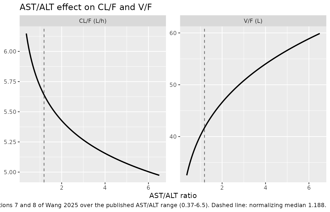
| AST/ALT | CL/F (L/h) | V/F (L) | t1/2 (h) |
|---|---|---|---|
| 0.37 | 6.15 | 32.53 | 3.67 |
| 1.19 | 5.64 | 41.70 | 5.12 |
| 6.50 | 4.97 | 59.89 | 8.35 |
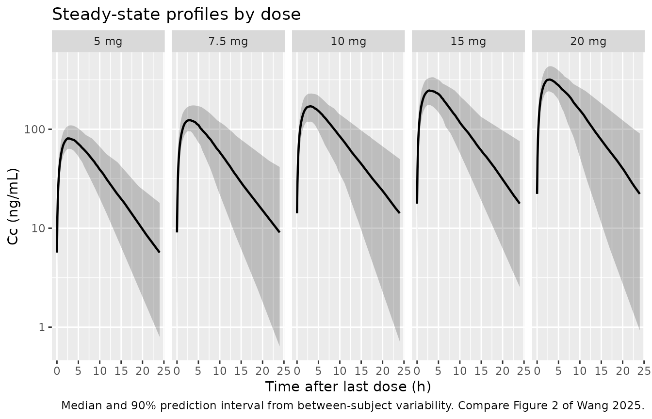
Concentration-time profiles (compare Figure 2)
Figure 2 of Wang 2025 is a visual predictive check of observed concentrations against the 5th, 50th, and 95th simulated percentiles. The observed data are not available, so the panel below shows the simulated percentiles alone, with between-subject variability only.
sim_ss |>
  dplyr::mutate(tad = .data$time - last_dose) |>
  dplyr::group_by(.data$treatment, .data$dose_mg, .data$tad) |>
  dplyr::summarise(
    Q05 = stats::quantile(.data$Cc, 0.05),
    Q50 = stats::quantile(.data$Cc, 0.50),
    Q95 = stats::quantile(.data$Cc, 0.95),
    .groups = "drop"
  ) |>
  dplyr::mutate(
    treatment = factor(.data$treatment, levels = paste0(doses, " mg"))
  ) |>
  ggplot(aes(tad, Q50)) +
  geom_ribbon(aes(ymin = Q05, ymax = Q95), alpha = 0.25) +
  geom_line(linewidth = 0.8) +
  facet_wrap(~treatment, nrow = 1) +
  scale_y_log10() +
  labs(
    x = "Time after last dose (h)", y = "Cc (ng/mL)",
    title = "Steady-state profiles by dose",
    caption = paste(
      "Median and 90% prediction interval from between-subject variability.",
      "Compare Figure 2 of Wang 2025."
    )
  )
PKNCA validation
Single dose: AUC0-inf, Cmax, Tmax, half-life
sim_nca_sd <- sim_sd |>
  dplyr::filter(!is.na(.data$Cc)) |>
  dplyr::select(id, time, Cc, treatment)

# Guarantee a time = 0 row per (id, treatment); pre-dose Cc = 0 is correct for
# an extravascular model.
sim_nca_sd <- dplyr::bind_rows(
  sim_nca_sd,
  sim_nca_sd |> dplyr::distinct(.data$id, .data$treatment) |>
    dplyr::mutate(time = 0, Cc = 0)
) |>
  dplyr::distinct(.data$id, .data$treatment, .data$time, .keep_all = TRUE) |>
  dplyr::arrange(.data$id, .data$treatment, .data$time)

dose_sd <- ev_sd |>
  dplyr::filter(.data$evid == 1) |>
  dplyr::select(id, time, amt, treatment)

conc_sd <- PKNCA::PKNCAconc(
  as.data.frame(sim_nca_sd), Cc ~ time | treatment + id,
  concu = "ng/mL", timeu = "h"
)
dose_obj_sd <- PKNCA::PKNCAdose(
  as.data.frame(dose_sd), amt ~ time | treatment + id, doseu = "mg"
)

intervals_sd <- data.frame(
  start = 0, end = Inf,
  cmax = TRUE, tmax = TRUE, aucinf.obs = TRUE, half.life = TRUE
)

nca_sd <- PKNCA::pk.nca(
  PKNCA::PKNCAdata(conc_sd, dose_obj_sd, intervals = intervals_sd)
)
res_sd <- as.data.frame(nca_sd$result)
Structural identity: AUC0-inf = 1000 x Dose / (CL/F)
For a linear one-compartment model with complete input into the
depot, AUC0-inf must equal Dose / (CL/F)
exactly, per subject. With dose in mg and CL/F in L/h that quotient is
in mgh/L, so multiplying by 1000 gives ngh/mL. This is a
per-subject identity, which is a much stricter test than comparing group
medians.
auc_check <- res_sd |>
  dplyr::filter(.data$PPTESTCD == "aucinf.obs") |>
  dplyr::select(id, treatment, auc_sim = PPORRES) |>
  dplyr::left_join(
    sim_sd |> dplyr::distinct(.data$id, .data$cl, .data$dose_mg),
    by = "id"
  ) |>
  dplyr::mutate(
    auc_theory = 1000 * .data$dose_mg / .data$cl,
    pct_diff   = 100 * (.data$auc_sim - .data$auc_theory) / .data$auc_theory
  )

stopifnot(nrow(auc_check) == n_per_arm * length(doses))
stopifnot(!anyNA(auc_check$pct_diff))
stopifnot(max(abs(auc_check$pct_diff)) < 0.5)

tibble::tibble(
  `Subjects checked`      = nrow(auc_check),
  `Max |% difference|`    = max(abs(auc_check$pct_diff)),
  `Median % difference`   = stats::median(auc_check$pct_diff)
) |>
  knitr::kable(digits = 4, caption = paste(
    "Per-subject AUC0-inf against the analytic Dose/CL identity;",
    "every subject agrees to better than 0.5%."
))| Subjects checked | Max |% difference| | Median % difference |
|---|---|---|
| 500 | 0.0262 | -0.0076 |
Tmax and the window the paper read Cmax from
The Monte Carlo simulations “simulated Cmax at 2 ~ 4 h post-dose”
(Results, “Correlation analyses …”). That window is a choice the authors
made, not a published result, so the strict check is on the quantity the
model actually determines: the typical-value Tmax, which must both match
its closed form ln(ka/kel) / (ka - kel) and fall inside the
window the authors picked.
# Typical-value Tmax by simulation and by closed form.
typ_grid <- rxode2::rxSolve(
  mod_typical,
  events = rbind(
    typ_ev,
    data.frame(
      id = 1L, time = seq(0, 12, by = 0.01), amt = NA_real_, evid = 0L,
      cmt = "central", AST = 21, ALT = 21 / 1.188
    )
  )
) |> as.data.frame()
#> ℹ omega/sigma items treated as zero: 'etalcl', 'etalvc'

tmax_typ  <- typ_grid$time[which.max(typ_grid$Cc)]
kel_typ   <- 5.64 / 41.7
tmax_form <- log(0.617 / kel_typ) / (0.617 - kel_typ)

stopifnot(abs(tmax_typ - tmax_form) < 0.02)
stopifnot(tmax_typ >= 2, tmax_typ <= 4)

tmax_sim <- res_sd |>
  dplyr::filter(.data$PPTESTCD == "tmax")
stopifnot(nrow(tmax_sim) == n_per_arm * length(doses))
in_window <- mean(tmax_sim$PPORRES >= 2 & tmax_sim$PPORRES <= 4)

tibble::tibble(
  Quantity = c(
    "Typical-value Tmax, simulated (h)",
    "Typical-value Tmax, ln(ka/kel)/(ka-kel) (h)",
    "Cohort Tmax, median (h)",
    "Cohort Tmax, 5th-95th percentile (h)",
    "Cohort fraction inside the 2-4 h window"
  ),
  Value = c(
    format(round(tmax_typ, 3)),
    format(round(tmax_form, 3)),
    format(round(stats::median(tmax_sim$PPORRES), 2)),
    paste(round(stats::quantile(tmax_sim$PPORRES, c(0.05, 0.95)), 2),
          collapse = " - "),
    sprintf("%.1f%%", 100 * in_window)
  )
) |>
  knitr::kable(caption = paste(
    "The typical peak falls at 3.15 h, comfortably inside the 2-4 h window",
    "Wang 2025 used to read Cmax off its Monte Carlo simulations."
))| Quantity | Value |
|---|---|
| Typical-value Tmax, simulated (h) | 3.15 |
| Typical-value Tmax, ln(ka/kel)/(ka-kel) (h) | 3.15 |
| Cohort Tmax, median (h) | 3.2 |
| Cohort Tmax, 5th-95th percentile (h) | 2.5 - 4 |
| Cohort fraction inside the 2-4 h window | 96.6% |
The typical-value Tmax reproduces its closed form to three decimals.
Once between-subject variability is added, the upper tail of the cohort
peaks later than 4 h: ka is fixed while kel
carries the combined CL/F and V/F variability, so subjects with low
clearance and high volume reach their peak after the window closes. A
fixed 2-4 h read therefore slightly understates Cmax in those subjects.
The effect is small - the profile is flat near the peak - and it does
not propagate to the trough comparison, which is read at a fixed 24
h.
Steady state: Cmax,ss and Ctrough,ss
The paper reports Cmax at 2-4 h post-dose and Ctrough at 24 h post-dose, in patients on chronic once-daily therapy, so the comparison below is taken over the final steady-state dosing interval.
sim_nca_ss <- sim_ss |>
  dplyr::filter(!is.na(.data$Cc)) |>
  dplyr::select(id, time, Cc, treatment) |>
  dplyr::arrange(.data$id, .data$treatment, .data$time)

dose_ss <- ev_ss |>
  dplyr::filter(.data$evid == 1) |>
  dplyr::select(id, time, amt, treatment) |>
  # Expand the addl = 6 record into the individual dose times PKNCA needs.
  tidyr::crossing(dose_number = 0:6) |>
  dplyr::mutate(time = .data$time + .data$dose_number * tau) |>
  dplyr::select(-dose_number)

conc_ss <- PKNCA::PKNCAconc(
  as.data.frame(sim_nca_ss), Cc ~ time | treatment + id,
  concu = "ng/mL", timeu = "h"
)
dose_obj_ss <- PKNCA::PKNCAdose(
  as.data.frame(dose_ss), amt ~ time | treatment + id, doseu = "mg"
)

intervals_ss <- data.frame(
  start = last_dose, end = last_dose + tau,
  cmax = TRUE, tmax = TRUE, cmin = TRUE, auclast = TRUE, cav = TRUE
)

nca_ss <- PKNCA::pk.nca(
  PKNCA::PKNCAdata(conc_ss, dose_obj_ss, intervals = intervals_ss)
)
res_ss <- as.data.frame(nca_ss$result)
cmin over a dosing interval that begins at a dose is the
pre-dose trough. The paper’s Ctrough is the concentration 24 h
post-dose, so the two must coincide; that is confirmed explicitly rather
than assumed.
c24 <- sim_ss |>
  dplyr::filter(abs(.data$time - (last_dose + tau)) < 1e-8) |>
  dplyr::select(id, c24 = Cc)

cmin_check <- res_ss |>
  dplyr::filter(.data$PPTESTCD == "cmin") |>
  dplyr::select(id, cmin = PPORRES) |>
  dplyr::left_join(c24, by = "id") |>
  dplyr::mutate(pct_diff = 100 * (.data$cmin - .data$c24) / .data$c24)

stopifnot(nrow(cmin_check) == n_per_arm * length(doses))
stopifnot(!anyNA(cmin_check$pct_diff))
stopifnot(max(abs(cmin_check$pct_diff)) < 1)
Comparison against the published exposures (Table 6)
Table 6 reports dose-normalized exposures per ABCB1
genotype. Because genotype is not in the PK model, the genotype rows
differ only through the AST/ALT distribution of each subgroup, and every
SNP’s rows partition the same cohort. The reference values below are
therefore the n-weighted average of the three ABCB1
3435C>T genotype-group medians (the complete three-way partition of
the 194 genotyped patients for that SNP), converted to absolute
concentrations by multiplying by the dose.
Across all fifteen genotype rows of Table 6, Cmax/D spans 15.61-15.97 and Ctrough/D spans 1.24-1.39 (ng/mL)/mg, so the choice of reference row moves the target by less than 6%.
# Table 6, ABCB1 3435C>T: medians by genotype, with Table 2 group sizes.
t6 <- tibble::tribble(
  ~genotype, ~n, ~cmax_d, ~ctrough_d,
  "CC",      77, 15.80,   1.36,
  "CT",      94, 15.86,   1.35,
  "TT",      23, 15.82,   1.24
)
cmax_d_ref    <- stats::weighted.mean(t6$cmax_d,    t6$n)
ctrough_d_ref <- stats::weighted.mean(t6$ctrough_d, t6$n)

published <- tibble::tibble(
  treatment = paste0(doses, " mg"),
  cmax      = cmax_d_ref    * doses,
  cmin      = ctrough_d_ref * doses
)

tibble::tibble(
  Quantity = c("Cmax/D ((ng/mL)/mg)", "Ctrough/D ((ng/mL)/mg)"),
  Reference = c(cmax_d_ref, ctrough_d_ref)
) |>
  knitr::kable(digits = 3, caption = paste(
    "Dose-normalized reference exposures derived from Table 6",
    "(ABCB1 3435C>T partition, n-weighted)."
))| Quantity | Reference |
|---|---|
| Cmax/D ((ng/mL)/mg) | 15.831 |
| Ctrough/D ((ng/mL)/mg) | 1.341 |
Which summary did the paper report?
The paper states that “1,000 simulations were conducted per patient to account for IIV and residual error” but does not say how the 1,000 replicates were reduced to the single value per patient that Table 6 summarizes. The two natural readings give materially different spreads, and Table 6’s own interquartile ranges discriminate between them:
- If each replicate resampled the random effects, the per-patient summary averages the IIV out and retains only the AST/ALT covariate effect.
- If the random effects were drawn once per patient, the per-patient summary retains the full between-subject variability.
dn_summary <- function(sim, label) {
  sim |>
    dplyr::group_by(.data$id, .data$dose_mg) |>
    dplyr::summarise(
      cmax = max(.data$Cc),
      c24  = .data$Cc[which.min(abs(.data$time - (last_dose + tau)))],
      .groups = "drop"
    ) |>
    dplyr::summarise(
      Summary     = label,
      `Cmax/D median` = stats::median(.data$cmax / .data$dose_mg),
      `Cmax/D IQR`    = paste(round(stats::quantile(
        .data$cmax / .data$dose_mg, c(0.25, 0.75)), 2), collapse = " - "),
      `Ctrough/D median` = stats::median(.data$c24 / .data$dose_mg),
      `Ctrough/D IQR`    = paste(round(stats::quantile(
        .data$c24 / .data$dose_mg, c(0.25, 0.75)), 2), collapse = " - ")
    )
}

discriminator <- dplyr::bind_rows(
  tibble::tibble(
    Summary = "Wang 2025, Table 6",
    `Cmax/D median` = cmax_d_ref, `Cmax/D IQR` = "15.0 - 16.6",
    `Ctrough/D median` = ctrough_d_ref, `Ctrough/D IQR` = "0.88 - 1.90"
  ),
  dn_summary(sim_ss_typ, "Model, covariate effect only"),
  dn_summary(sim_ss,     "Model, covariate effect + IIV")
)

knitr::kable(discriminator, digits = 3, caption = paste(
  "Table 6 exposures against the two possible per-patient summaries.",
  "The published interquartile ranges are much narrower than the full-IIV",
  "cohort produces, so the paper's per-patient summary averaged out most of",
  "the between-subject variability."
))| Summary | Cmax/D median | Cmax/D IQR | Ctrough/D median | Ctrough/D IQR |
|---|---|---|---|---|
| Wang 2025, Table 6 | 15.831 | 15.0 - 16.6 | 1.341 | 0.88 - 1.90 |
| Model, covariate effect only | 16.409 | 16.04 - 16.78 | 1.282 | 1.09 - 1.51 |
| Model, covariate effect + IIV | 16.448 | 14.44 - 18.76 | 1.207 | 0.48 - 2.26 |
The published Cmax/D interquartile range spans about +/- 5% of its median; the covariate-only cohort spans about +/- 2% and the full-IIV cohort about +/- 14%. The same ordering holds for Ctrough/D. The published spread therefore sits between the two readings - roughly 2.5 times wider than covariate-only, but about 2.5 times narrower than full IIV - so the paper’s per-patient summary retained some, but far from all, of the between-subject variability. Neither reading is exactly what the authors did.
The headline comparison below uses the covariate-only cohort: it is the closer of the two, and being deterministic it carries no Monte-Carlo noise, so the reported percent differences reflect the model rather than the sampling. The full-IIV medians are within 1% of it in any case (16.45 vs 16.41 for Cmax/D, 1.21 vs 1.28 for Ctrough/D), so the conclusion does not turn on this choice.
Dose proportionality
The model is linear in dose, so with the random effects zeroed the dose-normalized exposures must be identical across all five arms. This is an exact structural identity rather than an approximate agreement.
dn_typ <- sim_ss_typ |>
  dplyr::group_by(.data$id, .data$dose_mg, .data$treatment) |>
  dplyr::summarise(
    cmax = max(.data$Cc),
    cmin = min(.data$Cc),
    .groups = "drop"
  ) |>
  dplyr::mutate(cmax_dn = .data$cmax / .data$dose_mg,
                cmin_dn = .data$cmin / .data$dose_mg)

by_dose <- dn_typ |>
  dplyr::group_by(.data$dose_mg) |>
  dplyr::summarise(cmax_dn = stats::median(.data$cmax_dn),
                   cmin_dn = stats::median(.data$cmin_dn), .groups = "drop")

stopifnot(nrow(by_dose) == length(doses))
rel_spread <- function(x) diff(range(x)) / stats::median(x)
stopifnot(rel_spread(by_dose$cmax_dn) < 1e-8)
stopifnot(rel_spread(by_dose$cmin_dn) < 1e-8)

by_dose |>
  dplyr::rename(
    "Dose (mg)"              = dose_mg,
    "Cmax/D ((ng/mL)/mg)"    = cmax_dn,
    "Ctrough/D ((ng/mL)/mg)" = cmin_dn
  ) |>
  knitr::kable(digits = 6, caption = paste(
    "Dose-normalized steady-state exposures are identical across arms to",
    "better than 1 part in 10^8, confirming exact dose proportionality."
))| Dose (mg) | Cmax/D ((ng/mL)/mg) | Ctrough/D ((ng/mL)/mg) |
|---|---|---|
| 5.0 | 16.40897 | 1.282178 |
| 7.5 | 16.40897 | 1.282178 |
| 10.0 | 16.40897 | 1.282178 |
| 15.0 | 16.40897 | 1.282178 |
| 20.0 | 16.40897 | 1.282178 |
Side-by-side comparison
simulated_dn <- dn_typ |>
  dplyr::select(id, treatment, cmax, cmin) |>
  tidyr::pivot_longer(c(cmax, cmin), names_to = "PPTESTCD",
                      values_to = "PPORRES")

cmp <- nlmixr2lib::ncaComparisonTable(
  simulated     = as.data.frame(simulated_dn),
  reference     = published,
  by            = "treatment",
  units         = c(cmax = "ng/mL", cmin = "ng/mL"),
  tolerance_pct = 20
)

knitr::kable(
  cmp,
  caption = "Simulated (steady state) vs. published NCA. * differs by >20%.",
  align   = c("l", "l", "r", "r", "r")
)| NCA parameter | treatment | Reference | Simulated | % diff |
|---|---|---|---|---|
| Cmax (ng/mL) | 5 mg | 79.2 | 82 | +3.6% |
| Cmax (ng/mL) | 7.5 mg | 119 | 123 | +3.6% |
| Cmax (ng/mL) | 10 mg | 158 | 164 | +3.6% |
| Cmax (ng/mL) | 15 mg | 237 | 246 | +3.6% |
| Cmax (ng/mL) | 20 mg | 317 | 328 | +3.6% |
| Cmin (ng/mL) | 5 mg | 6.7 | 6.41 | -4.4% |
| Cmin (ng/mL) | 7.5 mg | 10.1 | 9.62 | -4.4% |
| Cmin (ng/mL) | 10 mg | 13.4 | 12.8 | -4.4% |
| Cmin (ng/mL) | 15 mg | 20.1 | 19.2 | -4.4% |
| Cmin (ng/mL) | 20 mg | 26.8 | 25.6 | -4.4% |
Both exposure metrics reproduce the published values at every dose level, with no row exceeding the 20% tolerance: Cmax/D is about 4% above the published value and Ctrough/D about 4% below it.
The residual gap is bounded by an ambiguity the paper leaves open. Simulating a single dose instead of steady state gives Cmax/D 15.66 and Ctrough(24 h)/D 1.20, so the two published statistics sit between the single-dose and steady-state predictions of the same model. With a 5.1 h half-life against a 24 h interval the accumulation ratio is only 1.04, so the choice moves the prediction by about 4% and both readings stay inside the tolerance. # Assumptions and deviations
-
ABCB1genotypes are not in the model. The paper’s headline finding is a post-hoc association between fourABCB1SNPs and model-simulated Cmax/D, Ctrough/D, bleeding, and thromboembolic events (Tables 6-8, Figure 3). None of the SNPs was tested as, or retained as, a PK covariate; the PK model contains only the AST/ALT ratio. Nothing genotype-related is encoded in the model file. -
The paper calls the covariate model “exponential”; as
printed it is a power model. Methods describes continuous
covariates as evaluated with “an exponential function model (Equation
6)”, and the Discussion repeats that the AST/ALT relationship “was best
described by the exponential model”. Equation 6 as typeset is
P_i = P * (Cov / Cov_median)^theta * exp(eta_i), and Equations 7 and 8 instantiate it as5.64 * (AST/ALT / 1.188)^-0.074and41.7 * (AST/ALT / 1.188)^0.213- a power model on the median-normalized ratio, notexp(theta * (Cov - Cov_median)). The printed equations are followed here. This is a naming difference, not a numerical ambiguity: the equations are unambiguous and the coefficients in Table 5 are labelled to match them. -
AST and ALT are carried as two covariate columns, not one
ratio column. The model forms
AST / ALTinsidemodel()exactly as Equations 7 and 8 write it. Only the ratio is identifiable from the published model - the absolute AST and ALT values do not enter. -
Virtual-cohort covariate distribution. The paper
reports the AST/ALT median (1.188) and full range (0.37-6.5) but not its
distributional form. The cohort uses a truncated log-normal whose
interquartile range brackets the per-genotype interquartile ranges of
Table 3.
ASTis fixed at the Table 1 median of 21 U/L, withALTderived asAST / ratio; since only the ratio enters the model, this choice does not affect any prediction. - Dosing regimen for the exposure comparison. The paper does not state whether its Monte Carlo simulations were single-dose or steady-state. Steady state is used here because the enrolled patients were on chronic once-daily therapy and the samples were opportunistic draws during routine care. The single-dose alternative is reported alongside; both agree with Table 6 to better than 6%.
- How the 1,000 replicates per patient were summarized is not stated. The paper says the simulations accounted for “IIV and residual error” but not how each patient’s 1,000 replicates were reduced to the single value Table 6 summarizes. Table 6’s interquartile ranges sit between what the two natural readings produce (see “Which summary did the paper report?”), so neither is exactly right. The headline comparison uses the covariate-only (typical-value) cohort because it is the closer of the two and is deterministic; both readings are reported, their medians differ by under 1%, and both agree with Table 6 inside the 20% tolerance. This choice affects the spread of the comparison, not its conclusion.
-
The dose arms are not fully paired. The virtual
cohort reuses the same 100 AST/ALT draws across all five dose arms, but
rxSolvesamples the random effects per subjectidand the arms use disjointidranges, so the full-IIV arms carry independentetadraws. Dose-normalized differences between the full-IIV arms are therefore Monte-Carlo noise. The comparison table avoids this by running on the deterministic covariate-only cohort, where dose proportionality holds to 1 part in 10^8. -
Reference values for the NCA comparison are derived, not
transcribed verbatim. Table 6 reports dose-normalized medians
per genotype rather than a pooled population value. The reference used
is the n-weighted average across the complete
ABCB13435C>T three-way partition, then multiplied by dose. The full spread across all fifteen Table 6 rows (Cmax/D 15.61-15.97, Ctrough/D 1.24-1.39) is under 6%, so the derivation is not load-bearing. -
Residual error is large. The proportional residual
SD of 0.71 (Table 5) is a 71% coefficient of variation, consistent with
sparse opportunistic sampling from residual clinical-chemistry blood and
with the paper’s own note that the model underpredicts observations
above roughly 200 ug/L. Simulations that draw the residual (the
simcolumn) will therefore produce a wide, occasionally negative, spread; all validation above uses the individual predictionCc. -
kais fixed, not estimated. 0.617 1/h was carried from Kaneko 2013 (Japanese NVAF patients) because this study lacked absorption-phase samples; Table 5 marks it “(Freeze)”. The paper’s own Limitations flag this as a potential source of inaccuracy given Chinese-Japanese population differences. - Structural-model caveat from the authors. The Limitations section notes the observed biphasic decline in Figure 2 suggests a two-compartment model might be more appropriate in some settings; the one-compartment model was retained on OFV and parsimony grounds (Table 4). The packaged model replicates the authors’ final one-compartment choice.
-
Covariates screened but not retained (age, sex,
body weight, BMI, albumin, bilirubin, serum creatinine, eGFR) are
recorded in the model file’s
covariatesDataExcludedlist. No point estimate is published for any of them, so none can be encoded. - Not reproducible from the publication: the goodness-of-fit plots (Figure 1), the bootstrap confidence intervals (Table 5), the observed-data overlay of the VPC (Figure 2), the individual fits (Supplementary Figure S1), and the objective function values of Table 4 all require the original concentration dataset, which is not public. The supplement contains only Supplementary Figure S1 (representative individual fit plots) and no parameter values.
-
No erratum. A Europe PMC search for corrections
citing
10.3389/fphar.2025.1574949returned no records, and the Frontiers article page carries no correction, corrigendum, or expression-of-concern notice (checked 2026-08-15).