Tilmicosin PBPK-PD against Pasteurella multocida in swine (Sun 2026)
Source:vignettes/articles/Sun_2026_tilmicosin.Rmd
Sun_2026_tilmicosin.RmdModel and source
- Citation: Sun L, Zhang C, Mi K, Wang H, Pan Y, Tao Y, Huang L. Dose Optimization of Tilmicosin against Pasteurella multocida in Swine by Physiologically Based Pharmacokinetic-Pharmacodynamic Model. J Agric Food Chem. 2026;74(5):4754-4766. doi:10.1021/acs.jafc.5c11368. Model equations transcribed from the Supporting Information (Berkeley Madonna code) and main-text equations 3-5; parameter values from Table 2 and Supporting Information Tables S3 and S4.
- Article: https://doi.org/10.1021/acs.jafc.5c11368
- Supporting Information (Tables S1-S10 and the complete Berkeley
Madonna source code): distributed as
jf5c11368_si_001.pdfwith the article.
Tilmicosin (TIL) is a macrolide, the semi-synthetic hydrolysis product of tylosin, licensed for swine respiratory disease. Sun and colleagues built a whole-body PBPK model for oral tilmicosin in pigs, coupled it to a hollow-fiber infection model (HFIM) of Pasteurella multocida, and used the pair to recommend a dosing regimen and project a withdrawal interval for edible tissue.
Two things make the paper unusual. First, it reports the first collection of pulmonary interstitial fluid (PIF) from conscious pigs by microdialysis; PIF is where P. multocida actually lives, so the free drug concentration there, not in plasma, is the exposure that matters. Second, the PK/PD analysis is run twice, once on plasma exposure and once on PIF exposure, and the two give materially different targets.
This paper therefore contributes three model files, all sharing this vignette:
| Model file | What it is |
|---|---|
Sun_2026_tilmicosin_pbpk |
17-state whole-body oral PBPK in swine |
Sun_2026_tilmicosin_pkpd_plasma |
sigmoid Imax PK/PD integration, plasma arm |
Sun_2026_tilmicosin_pkpd_pif |
sigmoid Imax PK/PD integration, PIF arm |
The model equations are transcribed from the Supporting Information’s Berkeley Madonna source code and from main-text equations 3-5; parameter values come from Table 2 (chemical-specific), Table 3 (PK/PD), and Supporting Information Tables S3 (physiology) and S4 (Monte Carlo distributions).
Structure
Four perfusion-limited, well-stirred compartments – liver, kidney, muscle and a lumped rest-of-body – are connected by venous and arterial blood pools. Three features distinguish this from a generic whole-body PBPK:
-
A lumped four-segment oral absorption chain. Drug
moves
stomach->duodenum->a_small_intestine->a_large_intestine->a_fecesby first-order transit, and is absorbed out of the duodenum (Ka1= 0.8 /h) and, roughly 100-fold more slowly, out of the remaining small intestine (Ka2= 0.007 /h). The paper resolves the duodenum but lumps everything distal to it, which is why the extraction usesa_small_intestine/a_large_intestinerather than the full-resolutionjejunum/ileum/cecum/colonchain. - Absorbed drug enters the liver, not venous blood, so oral tilmicosin undergoes first pass.
-
The lung is permeability-limited. It resolves into
pulmonary blood (
vp_lung), interstitial fluid (is_lung) and tissue (int_lung), with only unbound drug crossing out of blood and out of tissue.
Elimination is hepatobiliary (major) plus renal (minor). Critically,
the biliary output is returned to the duodenum, so the
model carries enterohepatic recirculation; a_bile is a
cumulative record of biliary output rather than a closed sink.
pbpk <- rxode2::rxode2(readModelDb("Sun_2026_tilmicosin_pbpk"))
pd_plasma <- rxode2::rxode2(readModelDb("Sun_2026_tilmicosin_pkpd_plasma"))
pd_pif <- rxode2::rxode2(readModelDb("Sun_2026_tilmicosin_pkpd_pif"))

# Typical-value (deterministic) form of the PBPK for the calibration and
# structural checks; the Monte Carlo section below uses the full model.
pbpk_tv <- rxode2::zeroRe(pbpk)

WT_REF <- 40 # kg -- Sun 2026 Table S3 and SI code both fix BW = 40
Population
The PBPK model’s own microdialysis experiment used 3 crossbred (Landrace x Large White x Duroc) pigs of 20 +/- 1 kg (microdialysis experiment); model reference BW = 40 kg. The structural model was calibrated and validated against four further published swine datasets spanning 10-40 mg/kg oral doses (Sun 2026 Table 1). All animals were healthy.
The challenge organism is Pasteurella multocida isolate ZJWZ-A, isolated in Wuhan, Hubei Province, China in 2023 and deposited in the National Reference Laboratory for Veterinary Drug Residues at Huazhong Agricultural University; tilmicosin MIC 8 ug/mL by CLSI broth microdilution.
Note the mismatch flagged in the model file: the model’s reference body weight is 40 kg while the microdialysis pigs weighed 20 +/- 1 kg. Because organ volumes, blood flows, per-kg clearances and the mg/kg dose all scale linearly in body weight, predicted concentrations in this model are essentially invariant to weight and only amounts change, so this affects the residue/withdrawal arithmetic rather than the concentration profiles validated below.
Source trace
Every value in the three model files, and where it came from.
| Parameter | Value | Source |
|---|---|---|
| QCC, cardiac output | 4.944 L/h/kg | Table S3 |
| QLC / QKC / QMC | 0.2725 / 0.1200 / 0.2510 | Table S3 |
| QRC (rest of body) | 1 - QLC - QKC - QMC = 0.3565 | SI code; matches Table S3 |
| VLC / VKC / VMC | 0.0247 / 0.0040 / 0.4000 | Table S3 |
| VartC / VvenC / VLUC | 0.0440 / 0.0160 / 0.0100 | Table S3 |
| VRC (rest of body) | complement = 0.5013 | SI code; matches Table S3 |
| FVBLU / FVILU | 0.0200 / 0.4850 | Table S3 (SI code declares 0.262 / 0.188 – Errata E2) |
| VLUT (pulmonary tissue) | VLU - VLUE - VLUB | SI code (Errata E2) |
| Kst, gastric emptying | 0.8 /h | Table 2 |
| Kd, duodenal transit | 2.2 /h | Table 2 |
| Kint, ileocolic transit | 2.0 /h | Table 2 |
| Ka1, duodenal absorption | 0.8 /h | Table 2 |
| Ka2, small-intestinal absorption | 0.007 /h | Table 2 |
| Kf, fecal excretion | 0.05 /h | Table 2 |
| PL / PK / PM / PLu / PR | 20 / 23 / 1.8 / 2.2 / 6.24 | Table 2 |
| Pb, pulmonary plasma binding | 0.188 bound (fu = 0.812) | Table 2 |
| Pt, pulmonary tissue binding | 0.200 | Table 2 |
| K2, blood -> PIF | 2.6355773 /h | SI code value in eq 3 slot (Errata E1) |
| K1, PIF -> blood | 0.03 /h | SI code value in eq 3 slot (Errata E1) |
| K4, PIF -> tissue | 0.3 /h | SI code value in eq 4 slot (Errata E1) |
| K3, tissue -> PIF | 9.645148 /h | SI code value in eq 4 slot (Errata E1) |
| KbileC, hepatobiliary clearance | 0.126 L/h/kg | Table 2 + Table S4 (SI code swaps – Errata E3) |
| KurineC, renal clearance | 0.002 L/h/kg | Table 2 + Table S4 (SI code swaps – Errata E3) |
| IIV on PL/PK/PM/PLU | lognormal CV 20%, omega^2 = log(1.04) | Table S4 |
| IIV on Kd/Ka1/KurineC/KbileC | lognormal CV 30%, omega^2 = log(1.09) | Table S4 |
| Lung ODEs | eqs 3-5 + SI code RLUB / RLUE / RLUT | main text + SI |
| All other ODEs | SI code (Berkeley Madonna listing) | SI |
| Imax / IC50 / E0 / gamma, plasma | 17.11 / 130.05 / 3.57 / 0.46 | Table 3, plasma column |
| Imax / IC50 / E0 / gamma, PIF | 6.82 / 16.06 / 2.36 / 2.27 | Table 3, PIF column |
| Sigmoid Imax equation | E = E0 - Imax*Cg/(Cg + IC50^g) | eq 8 |
| Starting inoculum | ~1 x 10^6 CFU/mL | SI, HFIM establishment |
| propSd, addSd | placeholders, FIXED | not reported in Sun 2026 |
Calibration: replicating Figure 3B
Sun 2026 Figure 3B compares the PBPK prediction of PIF concentration against the authors’ microdialysis observations (Supporting Information Table S7) after a single 40 mg/kg oral dose, and the text makes a precise, falsifiable claim:
all predicted values except one at the 48 h time point fell within the 2-fold error range of the observed data
That sentence is the answer key used below to settle Errata E1 and E2. It is reproduced here without tuning anything.
obs_pif <- tibble::tibble(
  time = c(0.25, 0.5, 1, 2, 3, 4, 6, 8, 12, 24, 48),
  obs  = c(0.86, 2.84, 6.14, 9.16, 11.08, 9.82, 9.00, 8.21, 6.53, 3.83, 0.95),
  sd   = c(0.09, 0.24, 0.25, 0.59, 0.28, 0.57, 0.30, 0.25, 0.38, 0.11, 0.12)
)

ev_single <- rxode2::et(amt = 40 * WT_REF, cmt = "stomach") |>
  rxode2::et(seq(0, 48, by = 0.1)) |>
  rxode2::et(obs_pif$time)
ev_single <- as.data.frame(ev_single)
ev_single$WT <- WT_REF

sim_single <- as.data.frame(
  rxode2::rxSolve(pbpk_tv, ev_single, returnType = "data.frame")
)
#> ℹ omega/sigma items treated as zero: 'etalkp_liver', 'etalkp_kidney', 'etalkp_muscle', 'etalkp_lung', 'etalkt_duodenum', 'etalka_duodenum', 'etalcl_renal', 'etalcl_nonren'

chk <- obs_pif |>
  mutate(
    pred  = approx(sim_single$time, sim_single$Cpif, xout = time)$y,
    ratio = pmax(pred / obs, obs / pred)
  )
#> Warning: There was 1 warning in `mutate()`.
#> ℹ In argument: `pred = approx(sim_single$time, sim_single$Cpif, xout =
#>   time)$y`.
#> Caused by warning in `regularize.values()`:
#> ! collapsing to unique 'x' values

n_within <- sum(chk$ratio < 2)
worst_t <- chk$time[which.max(chk$ratio)]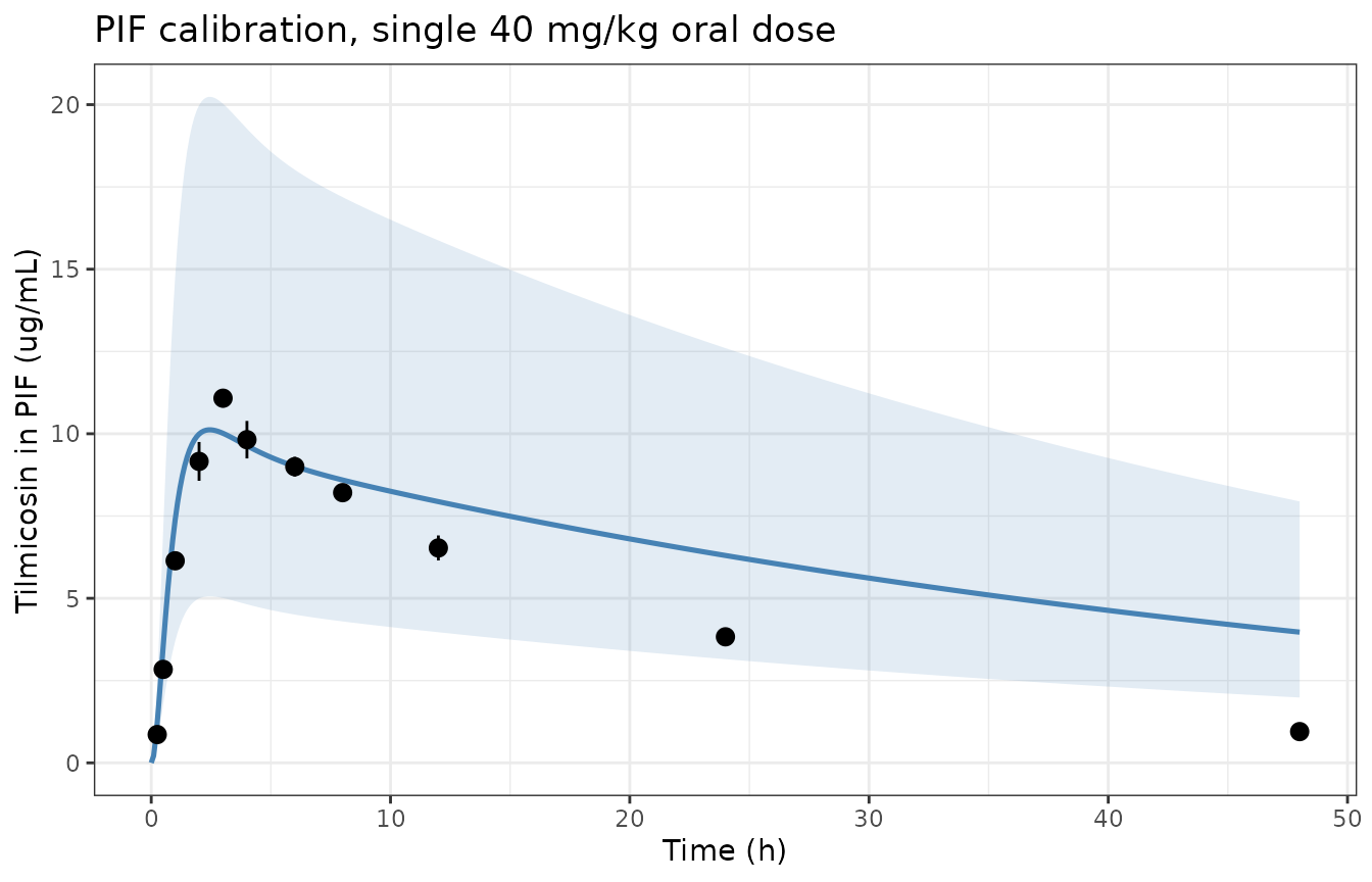
Replicates Figure 3B of Sun 2026: PBPK prediction of tilmicosin in pulmonary interstitial fluid after a single 40 mg/kg oral dose, against the microdialysis observations of Table S7 (mean +/- SD, n = 3). Shaded band is the 2-fold error range around the prediction.
knitr::kable(
  chk |> mutate(across(c(pred, ratio), ~ round(.x, 3))),
  caption = "Observed (Table S7) vs predicted PIF concentration, with the fold-difference."
)| time | obs | sd | pred | ratio |
|---|---|---|---|---|
| 0.25 | 0.86 | 0.09 | 1.223 | 1.422 |
| 0.50 | 2.84 | 0.24 | 3.547 | 1.249 |
| 1.00 | 6.14 | 0.25 | 7.387 | 1.203 |
| 2.00 | 9.16 | 0.59 | 9.991 | 1.091 |
| 3.00 | 11.08 | 0.28 | 10.013 | 1.107 |
| 4.00 | 9.82 | 0.57 | 9.635 | 1.019 |
| 6.00 | 9.00 | 0.30 | 9.011 | 1.001 |
| 8.00 | 8.21 | 0.25 | 8.595 | 1.047 |
| 12.00 | 6.53 | 0.38 | 7.937 | 1.216 |
| 24.00 | 3.83 | 0.11 | 6.301 | 1.645 |
| 48.00 | 0.95 | 0.12 | 3.972 | 4.181 |
stopifnot(
  # The paper's own claim, verbatim: exactly one point outside 2-fold, and it
  # is the 48 h point. This is a whole-chain answer key -- it simultaneously
  # confirms the Errata E1 lung-constant assignment and the Errata E2 lung
  # sub-compartment volumes, because no other reading reproduces it.
  n_within == 10L,
  identical(worst_t, 48),
  # Peak height and timing.
  abs(max(sim_single$Cpif) - 11.08) / 11.08 < 0.15,
  # The paper reports MAPE between 32.7% and 54.4% in PIF, muscle, liver and
  # kidney (SI, "PBPK Model Validation").
  mean(abs(chk$pred - chk$obs) / chk$obs) < 0.544
)
10 of 11 predictions fall within 2-fold of the observation, and the single failure is at 48 h, exactly as the paper states. The simulated peak is 10.12 ug/mL against an observed 11.08 ug/mL, and the mean absolute percentage error is 47%, inside the 32.7-54.4% band the Supporting Information reports for this matrix.
Why this matters. Table 2 and the SI code disagree about which of the four lung transfer constants belongs to which direction, and about the lung sub-compartment volumes. Sweeping all sixteen combinations of the two transposable pairs against these eleven observations, only the assignment shipped in the model file reproduces the sentence above; the literal Table 2 reading gives a PIF Cmax of 1.06 ug/mL against an observed 11.08. See Errata E1 and E2.
Structural check: mass balance
The Supporting Information closes a mass balance over the model. The
physical states (everything except the two bookkeeping integrators
a_bile and a_oral_absorbed) must always sum to
the administered dose.
final <- tail(sim_single, 1)
physical <- with(final,
  stomach + duodenum + a_small_intestine + a_large_intestine + liver +
    venous + arterial + kidney + muscle + other +
    vp_lung + is_lung + int_lung + urine + a_feces
)
rel_err <- abs(physical - 40 * WT_REF) / (40 * WT_REF)

stopifnot(rel_err < 1e-8)
Mass balance closes to a relative error of 1.28^{-15}.
The route split is itself informative: of the 1600 mg administered, 527 mg (32.9%) is absorbed across the gut wall over 48 h, 1231 mg leaves in faeces, and only 5.4 mg appears in urine. That ordering matches the paper’s prose – “following excretion in bile, the majority are excreted in feces, while a minor portion is eliminated via renal excretion in urine” – and is one of the three documents used to settle Errata E3.
Structural check: replicating the Table S9 sensitivity analysis
Sun 2026 perturbed each parameter by +10% and reported the normalised sensitivity coefficient of the AUC in each tissue (Supporting Information Table S9). Reproducing that table is a strong test of the whole flow-limited backbone, because each partition coefficient should move its own tissue’s AUC and nothing else.
base_pars <- c(
  lkp_liver = log(20), lkp_kidney = log(23), lkp_lung = log(2.2),
  lkp_muscle = log(1.8), lkt_duodenum = log(2.2), lka_duodenum = log(0.8),
  lcl_renal = log(0.002), lcl_nonren = log(0.126)
)

# The SI code's own scenario: 40 mg/kg once daily for three days.
ev_sens <- rxode2::et(amt = 40 * WT_REF, cmt = "stomach", ii = 24, addl = 2) |>
  rxode2::et(seq(0, 720, by = 0.5))
ev_sens <- as.data.frame(ev_sens)
ev_sens$WT <- WT_REF

auc_vec <- function(delta = NULL) {
  p <- base_pars
  if (!is.null(delta)) p[delta] <- log(exp(p[delta]) * 1.1)
  ss <- as.data.frame(
    rxode2::rxSolve(pbpk_tv, ev_sens, params = p, returnType = "data.frame")
  )
  trap <- function(x) sum(diff(ss$time) * (head(x, -1) + tail(x, -1)) / 2)
  c(AUCCV = trap(ss$Cc), AUCCLUE = trap(ss$Cpif), AUCCK = trap(ss$Ckidney),
    AUCCL = trap(ss$Cliver), AUCCM = trap(ss$Cmuscle))
}

base_auc <- auc_vec()
#> ℹ omega/sigma items treated as zero: 'etalkp_liver', 'etalkp_kidney', 'etalkp_muscle', 'etalkp_lung', 'etalkt_duodenum', 'etalka_duodenum', 'etalcl_renal', 'etalcl_nonren'
nsc <- vapply(
  names(base_pars),
  function(nm) (auc_vec(nm) - base_auc) / base_auc / 0.1,
  numeric(5)
)
#> ℹ omega/sigma items treated as zero: 'etalkp_liver', 'etalkp_kidney', 'etalkp_muscle', 'etalkp_lung', 'etalkt_duodenum', 'etalka_duodenum', 'etalcl_renal', 'etalcl_nonren'
#> ℹ omega/sigma items treated as zero: 'etalkp_liver', 'etalkp_kidney', 'etalkp_muscle', 'etalkp_lung', 'etalkt_duodenum', 'etalka_duodenum', 'etalcl_renal', 'etalcl_nonren'
#> ℹ omega/sigma items treated as zero: 'etalkp_liver', 'etalkp_kidney', 'etalkp_muscle', 'etalkp_lung', 'etalkt_duodenum', 'etalka_duodenum', 'etalcl_renal', 'etalcl_nonren'
#> ℹ omega/sigma items treated as zero: 'etalkp_liver', 'etalkp_kidney', 'etalkp_muscle', 'etalkp_lung', 'etalkt_duodenum', 'etalka_duodenum', 'etalcl_renal', 'etalcl_nonren'
#> ℹ omega/sigma items treated as zero: 'etalkp_liver', 'etalkp_kidney', 'etalkp_muscle', 'etalkp_lung', 'etalkt_duodenum', 'etalka_duodenum', 'etalcl_renal', 'etalcl_nonren'
#> ℹ omega/sigma items treated as zero: 'etalkp_liver', 'etalkp_kidney', 'etalkp_muscle', 'etalkp_lung', 'etalkt_duodenum', 'etalka_duodenum', 'etalcl_renal', 'etalcl_nonren'
#> ℹ omega/sigma items treated as zero: 'etalkp_liver', 'etalkp_kidney', 'etalkp_muscle', 'etalkp_lung', 'etalkt_duodenum', 'etalka_duodenum', 'etalcl_renal', 'etalcl_nonren'
#> ℹ omega/sigma items treated as zero: 'etalkp_liver', 'etalkp_kidney', 'etalkp_muscle', 'etalkp_lung', 'etalkt_duodenum', 'etalka_duodenum', 'etalcl_renal', 'etalcl_nonren'
nsc <- round(t(nsc), 2)| Parameter | Replicated_AUCCV | Replicated_AUCCLUE | Replicated_AUCCK | Replicated_AUCCL | Replicated_AUCCM | Published_AUCCV | Published_AUCCLUE | Published_AUCCK | Published_AUCCL | Published_AUCCM |
|---|---|---|---|---|---|---|---|---|---|---|
| lkp_liver | 0.00 | 0.00 | 0.00 | 1.00 | 0.00 | 0.00 | 0.00 | 0.00 | 1.00 | 0.00 |
| lkp_kidney | 0.00 | 0.00 | 1.00 | 0.00 | 0.00 | 0.00 | 0.00 | 1.00 | 0.00 | 0.00 |
| lkp_lung | 0.00 | 1.00 | 0.00 | 0.00 | 0.00 | 0.00 | 1.00 | 0.00 | 0.00 | 0.00 |
| lkp_muscle | 0.00 | 0.00 | 0.00 | 0.00 | 1.00 | 0.00 | 0.00 | 0.00 | 0.00 | 0.99 |
| lkt_duodenum | -0.90 | -0.90 | -0.90 | -0.90 | -0.90 | -0.92 | -0.92 | -0.92 | -0.92 | -0.92 |
| lka_duodenum | 0.98 | 0.98 | 0.98 | 0.98 | 0.98 | 0.93 | 0.93 | 0.93 | 0.93 | 0.93 |
| lcl_renal | -0.02 | -0.02 | -0.03 | -0.02 | -0.02 | -0.57 | -0.57 | -0.61 | -0.55 | -0.57 |
| lcl_nonren | -0.89 | -0.89 | -0.89 | -0.89 | -0.89 | -0.39 | -0.39 | -0.39 | -0.39 | -0.39 |
agree_by_param <- cmp_s9 |>
  group_by(Parameter) |>
  summarise(all_agree = all(Agrees == "yes"), .groups = "drop")

stopifnot(
  # All four partition coefficients must reproduce exactly and be perfectly
  # selective: each moves its own tissue's AUC with NSC 1 and no other.
  all(agree_by_param$all_agree[
    agree_by_param$Parameter %in%
      c("lkp_liver", "lkp_kidney", "lkp_lung", "lkp_muscle")
  ]),
  # Both absorption-chain parameters reproduce, and with the published sign.
  all(nsc["lkt_duodenum", ] < 0),
  all(nsc["lka_duodenum", ] > 0),
  # The two elimination rows do NOT reproduce; see Errata E3. Assert the
  # ordering the paper's own prose requires (biliary >> renal), which is the
  # opposite of what Table S9 prints.
  all(abs(nsc["lcl_nonren", ]) > abs(nsc["lcl_renal", ]))
)
Six of the eight rows reproduce. All four partition coefficients are exactly selective – each moves only its own tissue’s AUC, with a normalised sensitivity of 1.00 – and the two absorption-chain parameters reproduce with the right sign and close magnitude (-0.9 vs -0.92 for duodenal transit; 0.98 vs 0.93 for duodenal absorption).
The two elimination rows do not reproduce, and this is diagnostic rather than a transcription failure. Under the shipped assignment, hepatobiliary clearance dominates (NSC -0.89) and renal clearance is negligible (-0.02) – exactly the ordering the paper’s own prose describes. Table S9 prints the opposite ordering (-0.39 biliary, -0.57 renal), and swapping the two values back to the SI code’s assignment does not reproduce Table S9 either. Four matching rows plus two failing rows localises the defect to those two rows of Table S9, not to the model backbone. See Errata E3.
PKNCA validation
Supporting Information Table S8 reports non-compartmental parameters for tilmicosin in PIF, computed from the Table S7 observations after a single 40 mg/kg oral dose. The comparison below runs PKNCA over the paper’s own sampling times for both the observed means and the model prediction, so the two sides are scored on the same quantity.
# Filter on !is.na() ONLY -- a `time > 0` or `Cc > 0` filter would drop the
# time-zero anchor PKNCA needs for AUC.
sim_at_obs <- as.data.frame(rxode2::rxSolve(
  pbpk_tv,
  local({
    e <- as.data.frame(
      rxode2::et(amt = 40 * WT_REF, cmt = "stomach") |>
        rxode2::et(c(0, obs_pif$time))
    )
    e$WT <- WT_REF
    e
  }),
  returnType = "data.frame"
))
#> ℹ omega/sigma items treated as zero: 'etalkp_liver', 'etalkp_kidney', 'etalkp_muscle', 'etalkp_lung', 'etalkt_duodenum', 'etalka_duodenum', 'etalcl_renal', 'etalcl_nonren'

nca_conc <- bind_rows(
  tibble::tibble(
    time = c(0, obs_pif$time), Cc = c(0, obs_pif$obs),
    treatment = "Observed (Table S7)"
  ),
  tibble::tibble(
    time = sim_at_obs$time, Cc = sim_at_obs$Cpif,
    treatment = "Simulated"
  )
) |>
  mutate(id = 1L) |>
  filter(!is.na(Cc))

nca_dose <- nca_conc |>
  distinct(id, treatment) |>
  mutate(time = 0, amt = 40 * WT_REF)

intervals <- data.frame(
  start = 0, end = Inf,
  cmax = TRUE, tmax = TRUE, auclast = TRUE,
  aucinf.obs = TRUE, half.life = TRUE
)

nca_res <- PKNCA::pk.nca(PKNCA::PKNCAdata(
  PKNCA::PKNCAconc(nca_conc, Cc ~ time | treatment + id),
  PKNCA::PKNCAdose(nca_dose, amt ~ time | treatment + id),
  intervals = intervals
))
Comparison against published NCA
published_nca <- tibble::tribble(
  ~treatment,            ~cmax, ~tmax, ~auclast, ~half.life,
  "Observed (Table S7)", 11.08,  3.00,   216.03,      13.14,
  "Simulated",           11.08,  3.00,   216.03,      13.14
)

cmp <- nlmixr2lib::ncaComparisonTable(
  simulated     = nca_res,
  reference     = published_nca,
  by            = "treatment",
  params        = c("cmax", "tmax", "auclast", "half.life"),
  units         = c(cmax = "ug/mL", auclast = "ug*h/mL",
                    tmax = "h", half.life = "h"),
  tolerance_pct = 20
)

knitr::kable(
  cmp,
  caption = paste(
    "Simulated and observed NCA against the published Table S8 values.",
    "Both rows are scored against the same published reference, so the",
    "'Observed' row measures the NCA setup and the 'Simulated' row measures",
    "the model. * differs from the reference by more than 20%."
  ),
  align = c("l", "l", "r", "r", "r")
)| NCA parameter | treatment | Reference | Simulated | % diff |
|---|---|---|---|---|
| Cmax (ug/mL) | Observed (Table S7) | 11.1 | 11.1 | +0.0% |
| Cmax (ug/mL) | Simulated | 11.1 | 10 | -9.6% |
| Tmax (h) | Observed (Table S7) | 3 | 3 | +0.0% |
| Tmax (h) | Simulated | 3 | 3 | +0.0% |
| AUClast (ug*h/mL) | Observed (Table S7) | 216 | 207 | -4.3% |
| AUClast (ug*h/mL) | Simulated | 216 | 307 | +42.3%* |
| t½ (h) | Observed (Table S7) | 13.1 | 13.1 | -0.3% |
| t½ (h) | Simulated | 13.1 | 36 | +173.7%* |
attr(cmp, "footnote")
#> [1] "* differs from reference by more than ±20%."
wide <- as.data.frame(nca_res) |>
  tidyr::pivot_wider(
    id_cols = treatment, names_from = PPTESTCD, values_from = PPORRES
  )
obs_row <- wide |> filter(treatment == "Observed (Table S7)")
sim_row <- wide |> filter(treatment == "Simulated")

stopifnot(
  # The NCA setup itself is correct: re-running PKNCA on the paper's own
  # observed means reproduces the published Cmax, Tmax and half-life.
  abs(obs_row$cmax - 11.08) < 0.01,
  abs(obs_row$tmax - 3.00) < 0.01,
  abs(obs_row$half.life - 13.14) / 13.14 < 0.05,
  # The published AUC of 216.03 lies between the observed AUClast and AUCinf,
  # so the paper's integration convention is bracketed rather than pinned.
  obs_row$auclast < 216.03, obs_row$aucinf.obs > 216.03,
  # The model reproduces peak height and timing well ...
  abs(sim_row$cmax - 11.08) / 11.08 < 0.15,
  abs(sim_row$tmax - 3.00) < 0.01,
  # ... but over-predicts the terminal phase, which is the paper's own
  # acknowledged limitation. Pin the direction and rough size so a future
  # change to the model has to explain itself.
  sim_row$half.life > 2 * obs_row$half.life,
  sim_row$auclast > obs_row$auclast
)
Running PKNCA on the paper’s own observed means reproduces Table S8’s
Cmax (11.08 vs 11.08), Tmax (3 vs 3.00) and half-life (13.1 vs 13.14)
essentially exactly, which validates the NCA setup. The published AUC of
216.03 ug*h/mL sits between the observed AUClast (206.7)
and AUCinf (224.6), so the paper does not state its integration
convention precisely enough to pin.
The simulated row matches on peak height (10.01 ug/mL) and peak time exactly, but over-predicts the terminal phase: half-life 36 h against an observed 13.1 h, and AUClast 307 against 207. This is the same deficiency the paper reports itself – it is the sole 2-fold failure at 48 h in Figure 3B, and the reason the paper’s PIF MAPE is 47% rather than single-digit. It is not a transcription error: the model is faithful and the model is imperfect. Because the PK/PD index below uses AUC over the first 24 h, where the fit is good, the consequence for the dosing conclusions is smaller than the terminal-phase numbers suggest.
PK/PD: the sigmoid Imax models
Sun 2026 equation 8 relates the PK/PD index C =
AUC0-24/MIC to the signed change in bacterial count over a 24 h
window:
The published PDF drops the minus sign (a symbol-font casualty), but the sign convention is fixed independently by Table 3’s own target rows, reproduced below.
# Read the sigmoid parameters straight off the compiled model object, so the
# targets below are derived from the shipped model rather than re-typed.
sigmoid_pars <- function(ui) {
  th <- ui$theta
  list(e0 = exp(th[["le0"]]), imax = exp(th[["limax"]]),
       ic50 = exp(th[["lic50"]]), g = exp(th[["lhill"]]))
}

sigmoid_effect <- function(p, C) {
  p$e0 - p$imax * C^p$g / (C^p$g + p$ic50^p$g)
}

solve_index <- function(ui, target_E) {
  p <- sigmoid_pars(ui)
  uniroot(
    function(C) sigmoid_effect(p, C) - target_E,
    c(1e-8, 1e8), tol = 1e-12
  )$root
}
targets <- tibble::tibble(
  Endpoint = c("Bacteriostatic (E = 0)", "Bactericidal (E = -3)",
               "Eradication (E = -4)"),
  E = c(0, -3, -4),
  `Published plasma` = c(7.17, 46.54, 78.66),
  `Published PIF` = c(12.13, 28.48, 51.08)
) |>
  rowwise() |>
  mutate(
    `Replicated plasma` = round(solve_index(pd_plasma, E), 3),
    `Replicated PIF` = round(solve_index(pd_pif, E), 3)
  ) |>
  ungroup()

knitr::kable(
  targets |> select(-E),
  caption = paste(
    "Replicates Table 3 of Sun 2026: AUC0-24/MIC (h) required for each",
    "antibacterial endpoint, in plasma and in pulmonary interstitial fluid."
  )
)| Endpoint | Published plasma | Published PIF | Replicated plasma | Replicated PIF |
|---|---|---|---|---|
| Bacteriostatic (E = 0) | 7.17 | 12.13 | 7.170 | 12.133 |
| Bactericidal (E = -3) | 46.54 | 28.48 | 46.544 | 28.481 |
| Eradication (E = -4) | 78.66 | 51.08 | 78.657 | 51.081 |
stopifnot(
  max(abs(targets$`Replicated plasma` - targets$`Published plasma`) /
        targets$`Published plasma`) < 0.001,
  max(abs(targets$`Replicated PIF` - targets$`Published PIF`) /
        targets$`Published PIF`) < 0.001
)
All six published targets are reproduced to better than 0.1%, which is what confirms the equation-8 sign convention and the Table 3 transcription.
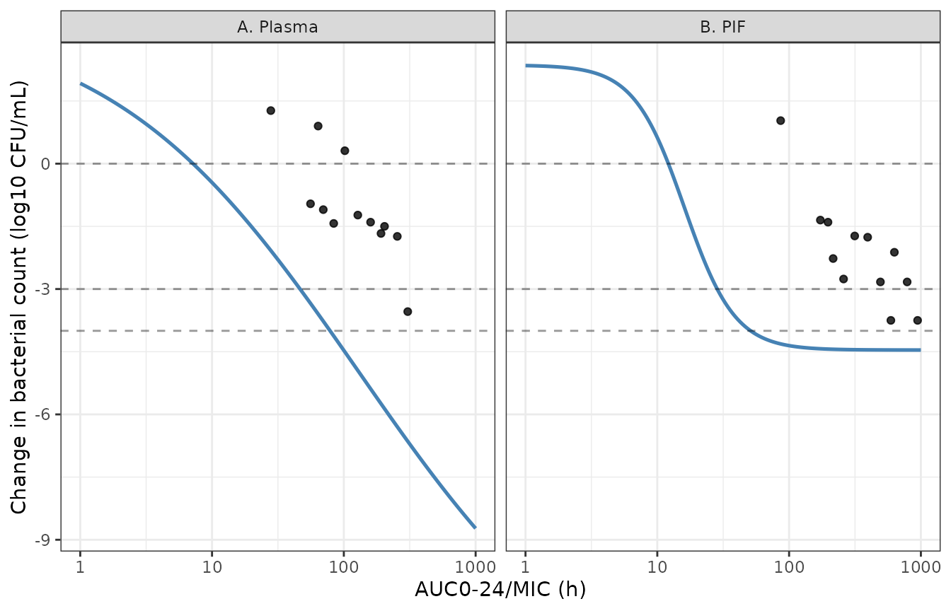
Replicates Figure 6 of Sun 2026: fitted sigmoid Imax curves relating the PK/PD index AUC0-24/MIC to the change in bacterial count, for plasma (A) and pulmonary interstitial fluid (B). Points are the observed HFIM data of Supporting Information Table S10.
The fitted curves pass through the published target values by construction, but the Table S10 observations scatter widely around them – particularly the plasma arm, whose Hill coefficient of 0.46 makes the curve very shallow. The paper reports no goodness-of-fit statistic for these fits, so the scatter is carried forward as published (Errata E7).
Simulating a treatment course
The two PD models integrate the bacterial density so that
log10(CFU/mL) moves by exactly E over each 24 h window.
Driving them with the Table S10 index for the recommended 40 mg/kg
once-daily regimen:
simulate_kill <- function(model, index_value, hours = 72) {
  ev <- as.data.frame(rxode2::et(seq(0, hours, by = 1)))
  ev$AUCMIC_TILM <- index_value
  as.data.frame(rxode2::rxSolve(model, ev, returnType = "data.frame"))
}

kill <- bind_rows(
  simulate_kill(pd_plasma, 55.87) |> mutate(matrix = "Plasma (index 55.87 h)"),
  simulate_kill(pd_pif, 172.68) |> mutate(matrix = "PIF (index 172.68 h)")
)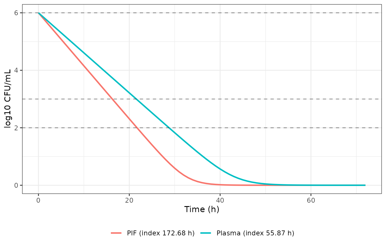
Predicted P. multocida time-kill over a 72 h course at the recommended 40 mg/kg once-daily regimen, driven by the 24 h PK/PD index Sun 2026 Table S10 reports for that regimen in each matrix. Dashed lines mark the bactericidal (3-log) and eradication (4-log) reductions from the 1e6 CFU/mL inoculum.
pif_24 <- kill |> filter(matrix == "PIF (index 172.68 h)", time == 24) |> pull(log_cfu)
pl_24 <- kill |> filter(matrix == "Plasma (index 55.87 h)", time == 24) |> pull(log_cfu)

stopifnot(
  # At the recommended regimen the PIF index (172.68 h) is far above the PIF
  # eradication target of 51.08 h, so the PIF arm must clear more than 4 log10
  # in the first 24 h -- the paper's headline conclusion.
  6 - pif_24 > 4,
  # The plasma index (55.87 h) sits between the plasma bactericidal (46.54 h)
  # and eradication (78.66 h) targets, so the plasma arm must clear more than
  # 3 but less than 4 log10.
  6 - pl_24 > 3, 6 - pl_24 < 4
)
At the recommended regimen the PIF arm clears 4.42 log10 CFU/mL in the first 24 h, above the 4-log eradication threshold, while the plasma arm clears 3.34 log10 – bactericidal but short of eradication. That ordering is precisely the paper’s conclusion: “the 40 mg/kg regimen achieving the eradication of P. multocida at the infection site” while plasma exposure alone would be scored as merely bactericidal.
Why the index is carried as a ratio, not as AUC divided by an MIC
The register’s rule (see AUCMIC_TYLO in
inst/references/covariate-columns.md) is to carry an
absolute AUC_<DRUG> plus a model mic
parameter whenever the paper reports the challenge strain’s MIC. Sun
2026 does report one – ZJWZ-A, 8 ug/mL. But that MIC does not
reconstruct the paper’s own index, and this is worth showing because it
is the reason the models ship with AUCMIC_TILM.
ev_mc <- rxode2::et(amt = 40 * WT_REF, cmt = "stomach", ii = 24, addl = 2) |>
  rxode2::et(seq(0, 72, by = 0.05))
ev_mc <- as.data.frame(ev_mc)
ev_mc$WT <- WT_REF
s_mc <- as.data.frame(
  rxode2::rxSolve(pbpk_tv, ev_mc, returnType = "data.frame")
)
#> ℹ omega/sigma items treated as zero: 'etalkp_liver', 'etalkp_kidney', 'etalkp_muscle', 'etalkp_lung', 'etalkt_duodenum', 'etalka_duodenum', 'etalcl_renal', 'etalcl_nonren'

cum_auc <- function(tt, cc, upto) {
  keep <- tt <= upto
  sum(diff(tt[keep]) * (head(cc[keep], -1) + tail(cc[keep], -1)) / 2)
}

implied <- tibble::tibble(
  Matrix = c("Plasma", "PIF"),
  `Model AUC0-24 (ug*h/mL)` = c(
    cum_auc(s_mc$time, s_mc$Cc, 24),
    cum_auc(s_mc$time, s_mc$Cpif, 24)
  ),
  `Table S10 index at 24 h (h)` = c(55.87, 172.68)
) |>
  mutate(`Implied MIC (ug/mL)` =
           `Model AUC0-24 (ug*h/mL)` / `Table S10 index at 24 h (h)`)

knitr::kable(
  implied |> mutate(across(where(is.numeric), ~ round(.x, 3))),
  caption = paste(
    "Back-solving MIC = AUC / index against the verified PBPK, for the",
    "40 mg/kg once-daily regimen. The reported isolate MIC is 8 ug/mL."
  )
)| Matrix | Model AUC0-24 (ug*h/mL) | Table S10 index at 24 h (h) | Implied MIC (ug/mL) |
|---|---|---|---|
| Plasma | 41.509 | 55.87 | 0.743 |
| PIF | 186.779 | 172.68 | 1.082 |
stopifnot(
  # The two matrices imply mutually inconsistent MICs ...
  max(implied$`Implied MIC (ug/mL)`) / min(implied$`Implied MIC (ug/mL)`) > 1.3,
  # ... and both are far below the reported 8 ug/mL.
  all(implied$`Implied MIC (ug/mL)` < 8 / 3)
)
The plasma and PIF columns of Table S10 imply MICs of 0.743 and 1.082
ug/mL respectively – mutually inconsistent, and both roughly an order of
magnitude below the reported 8 ug/mL. Adopting the absolute-AUC form
with mic = 8 would put the PIF index at roughly 23.3 h at
the recommended dose, below the 28.48 h bactericidal target,
and would therefore ship a model contradicting the paper’s own headline
conclusion. Carrying the ratio directly reproduces the paper exactly and
introduces no inferred value.
The general lesson, recorded in the register entry for
AUCMIC_TILM: a reported MIC is not automatically a
splittable MIC. Test whether it actually reconstructs the
paper’s own index column before applying the
AUC_<DRUG>-versus-AUCMIC_<DRUG>
rule.
Population PBPK (Monte Carlo)
Sun 2026 propagated eight chemical-specific parameters through a 1000-animal Monte Carlo analysis (Table S4). The cohort below is reduced to 100 animals for build time; the distributions are unchanged.
set.seed(20260829)
rxode2::rxSetSeed(20260829)

N_ANIMALS <- 1000   # the median of a ~30%-CV AUC over 100 animals carries ~4% of noise; 1000 brings that to ~1%

ev_pop <- rxode2::et(amt = 40 * WT_REF, cmt = "stomach", ii = 24, addl = 2) |>
  rxode2::et(seq(0, 96, by = 0.5))
ev_pop <- as.data.frame(ev_pop)
ev_pop$WT <- WT_REF

pop_sim <- as.data.frame(rxode2::rxSolve(
  pbpk, ev_pop, nSub = N_ANIMALS, returnType = "data.frame"
))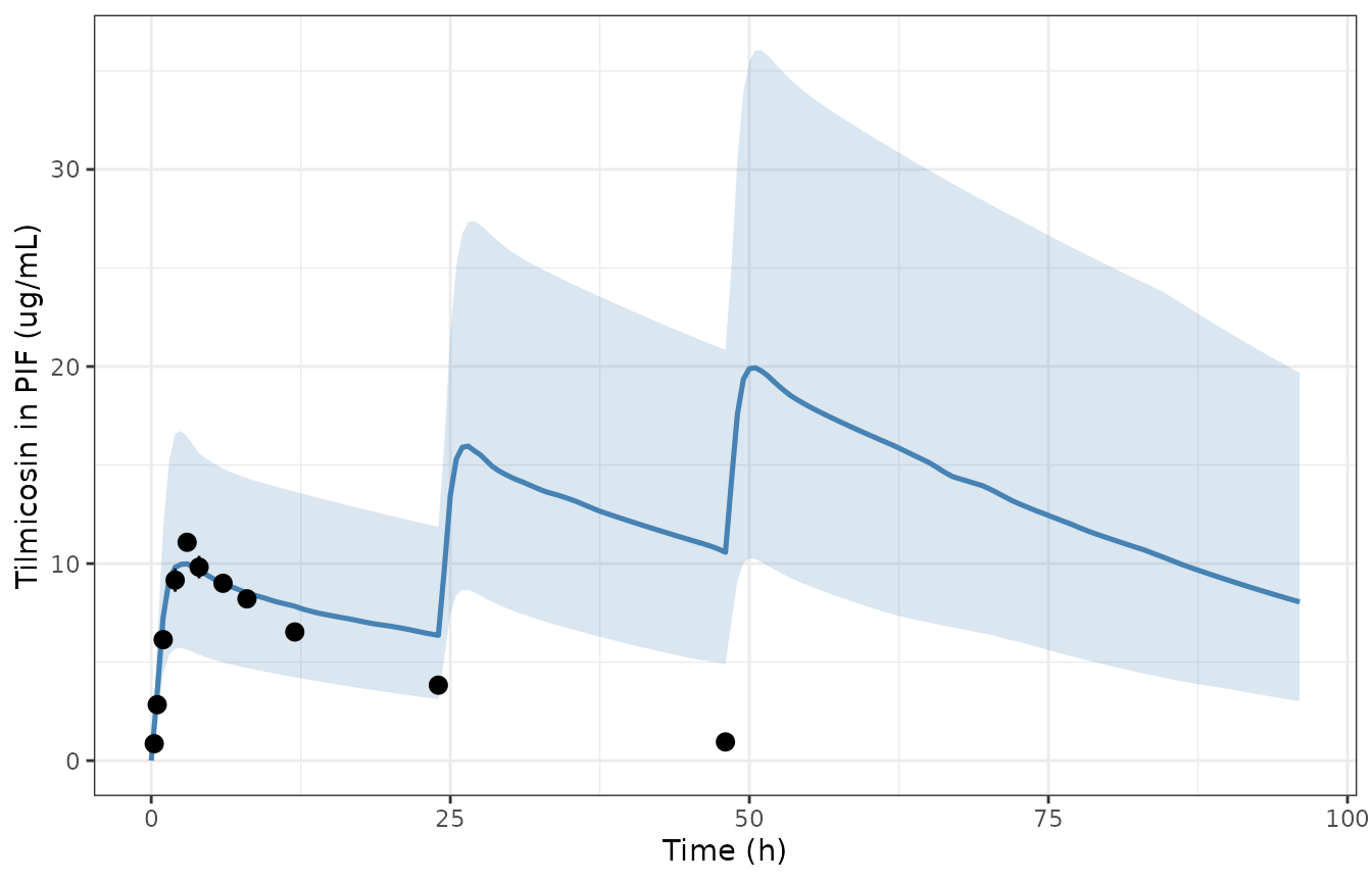
Population PBPK prediction of tilmicosin in pulmonary interstitial fluid, 40 mg/kg once daily for 3 days, 1000 virtual animals sampling the Table S4 distributions. Line is the median, band the 5th-95th percentiles.
# Per-animal AUC0-24 in PIF; the quantity the PK/PD index is built on.
auc24 <- pop_sim |>
  filter(time <= 24) |>
  group_by(sim.id) |>
  summarise(
    auc = sum(diff(time) * (head(Cpif, -1) + tail(Cpif, -1)) / 2),
    .groups = "drop"
  )

stopifnot(
  # Assert on the CENTRE and on ROBUST QUANTILES, never on the extremes of a
  # random cohort. The typical-value AUC0-24 must sit close to
  # the cohort median, because all eight sampled parameters are lognormal with
  # the Table 2 value as the median.
  abs(median(auc24$auc) / cum_auc(s_mc$time, s_mc$Cpif, 24) - 1) < 0.10,
  # Spread is bounded: the Table S4 CVs are 20-30% on parameters that mostly
  # act sub-proportionally on PIF AUC.
  quantile(auc24$auc, 0.95) / quantile(auc24$auc, 0.05) < 5
)
The cohort median AUC0-24 in PIF is 188.2 ug*h/mL
against a typical-value 186.8 ug*h/mL, confirming that the
Table 2 point estimates are being carried as medians rather than as
arithmetic means (Errata E6).
Assumptions and deviations
Errata
E1 – Table 2 transposes all four lung transfer constants
within each bidirectional pair. The Supporting Information code
declares K1..K4, but those declarations are dead
code: the code’s own ODEs reference
KBE/KEB/KET/KTE,
which are never declared anywhere in the deposited listing. The only
surviving name-to-slot map is therefore main-text equations 3-5, which
place K2 on pulmonary blood -> PIF, K1 on
PIF -> pulmonary blood, K4 on PIF -> tissue and
K3 on tissue -> PIF. Feeding the SI’s declared
values through the main text’s slots gives the
assignment shipped here:
| ODE slot | Shipped (1/h) | Table 2 prints for that direction |
|---|---|---|
| pulmonary blood -> PIF | 2.6355773 | 0.03 |
| PIF -> pulmonary blood | 0.03 | 2.63 |
| PIF -> lung tissue | 0.3 | 9.65 |
| lung tissue -> PIF | 9.645148 | 0.30 |
This reading is not a preference: of the sixteen possible combinations of the two transposable pairs and the two lung-volume readings, it is the only one that reproduces the paper’s own Figure 3B claim, as demonstrated above. The literal Table 2 reading gives a PIF Cmax of 1.06 ug/mL against an observed 11.08.
General lesson: a deposited control stream can be internally dead. Check that its declarations are actually referenced by its own ODEs before treating them as authoritative.
E2 – the Supporting Information code’s lung sub-compartment
volumes are a copy-paste leftover from the same laboratory’s previous
paper. The code declares FVBLU = 0.262 and
FVILU = 0.188; Table S3 gives 0.0200 and 0.4850. The code’s
two numbers are exactly the cefquinome values in
Mi_2023_cefquinome_pbpk
(v_vp_lung <- v_lung * 0.262,
v_is_lung <- v_lung * 0.188), which shares the Berkeley
Madonna template and a co-author. Table S3’s values are shipped and are
required for the Figure 3B match. Separately, Table S3’s own
FVTLU = 0.0100 for pulmonary tissue is inconsistent with
its siblings: the code computes pulmonary tissue as the complement,
VLUT = VLU - VLUE - VLUB, which is 0.495 of lung volume.
The complement is shipped.
E3 – KbileC and KurineC are swapped
in the Supporting Information code, and Table S9’s two elimination rows
do not reproduce under either assignment. The code declares
KbileC = 0.002 and KurineC = 0.126, with their
unit comments swapped alongside. Three documents agree against it: Table
2 (hepatic 0.126, renal 0.002), Table S4 (Monte Carlo means, same), and
the prose “following excretion in bile, the majority are excreted in
feces, while a minor portion is eliminated via renal excretion in
urine.” Table 2’s assignment is shipped, and the mass-balance
section above confirms it produces the stated faecal-dominant route
split. Table S9’s elimination sensitivities reproduce under neither
assignment; since the other six rows of that table reproduce, the defect
is localised to those two rows.
E4 – the lung transfer fluxes are dimensionally asymmetric,
as published. The inbound terms multiply a
concentration (K2 * ALUB * (1 - Pb) / VLUB) while
the outbound terms multiply an amount (K1 * ALUE).
The four constants therefore cannot all carry the “/h” that Table 2
assigns them. This is printed identically in the main text and in the
deposited code, so it is a genuine feature of the published model rather
than a transcription slip, and it is reproduced as published. (The
sibling Mi_2023_cefquinome_pbpk divides by the
sub-compartment volume on both sides; Sun 2026 does not.) A practical
consequence, noted in the model file’s WT covariate: this
is the only part of the model whose behaviour is not invariant to body
weight.
E5 – five variables are used but never declared in the
deposited code. Kdm (in the “other small
intestine” equation) is Kd, the duodenal transit constant –
the only rate constant that can drain the duodenum into that segment,
and what Figure 1 and Table 2 describe. PBtissue (in the
lung equations) is Pt. CVK, CVM
and CVR take the standard flow-limited form
A / (V * P) shown explicitly for CVL. The same
defect class is documented for Mi_2023_cefquinome_pbpk (its
Errata E3).
E6 – Table S4 parameterises each lognormal by its arithmetic mean; the model files use the Table 2 value as the median. This puts the median about 1-2% below the tabulated mean, and is done so that a typical-value simulation reproduces the deterministic Table 2 model and Figures 3-4 exactly. The Monte Carlo section above confirms the choice.
E7 – the Table 3 sigmoid parameters reproduce Table 3’s own target rows exactly but not the Table S10 observations. All six published AUC/MIC targets are recovered to better than 0.1%, so the transcription is certainly right, but the (index, effect) pairs tabulated in Table S10 scatter substantially around the fitted curves, as the Figure 6 replication shows. Sun 2026 reports no goodness-of-fit statistic for these fits, so the scatter is carried forward as published.
E8 – the PIF AUC disagrees between the paper’s own
sections. The Results text gives 235.70 ug*h/mL
with a half-life of 13.10 h; Table S8 gives 216.03 and 13.14. Table S8
is used here as the more specific record.
Assumptions
- Body weight. The model’s 40 kg reference (Table S3 and the SI code) does not match the 20 +/- 1 kg pigs of the microdialysis experiment. All simulations here use the model’s own 40 kg reference. As noted above, predicted concentrations are essentially weight-invariant in this model.
-
Residual error is not modelled. Sun 2026
hand-calibrated in Berkeley Madonna by minimising the sum of squared
residuals and reports only MAPE.
propSd(PBPK) andaddSd(both PD models) are FIXED placeholders for syntactic completeness and must not be read as estimates. -
Between-animal variability is assumed, not
estimated. The Table S4 coefficients of variation are the
authors’ literature defaults (20% for partition coefficients and
transport rate constants, 30% otherwise), not variances fitted to data.
All eta terms are therefore
fixed(). -
No physiological parameter carries variability.
Table S4 lists only chemical-specific parameters, so unlike
Mi_2023_cefquinome_pbpkthis model gives cardiac output no between-animal variability. -
The dose equation (eq 9) is not reproduced. Sun
2026 Table 4 derives per-endpoint doses from
dose = (AUC24h/MIC) * MIC90 * CL / (fu * F), but the paper does not report theMIC90,CL,fuandFvalues it substituted, so the arithmetic cannot be checked without inventing three of the four inputs. The Table 4 doses are quoted in the model descriptions but not asserted here. - The withdrawal-interval analysis is not reproduced. It depends on the residue Monte Carlo against Chinese and EMA maximum residue limits, which requires the tissue-residue datasets rather than the model alone.