Amphotericin B in rats (Santos 2024)
Source:vignettes/articles/Santos_2024_amphotericinB_rat.Rmd
Santos_2024_amphotericinB_rat.RmdModel and source
ui <- rxode2::rxode(readModelDb("Santos_2024_amphotericinB_rat"))
#> ℹ parameter labels from comments will be replaced by 'label()'- Citation: Santos VV, Pereira LC, de Araujo JMS, Borges MAH, Brandao CM, Santos LO, Villarreal CF, Azeredo FJ. Amphotericin B tissue penetration and pharmacokinetics in healthy and Candida albicans-infected rats: insights from microdialysis and population modeling. Front Pharmacol. 2024;15:1515462. doi:10.3389/fphar.2024.1515462
- Description: Preclinical (rat). Two-compartment population PK model for intravenous amphotericin B deoxycholate in healthy and Candida albicans-infected Wistar rats, fitted jointly to total plasma and microdialysis free kidney concentrations, with the peripheral compartment representing the kidney. The ODEs are the paper’s printed Equations 5-6, which carry a 0.56 factor on the kidney inflow only; with the published estimates this structure does not conserve mass and does not reproduce the paper’s figures or NCA AUCs (see the vignette) (Santos 2024)
- Article: https://doi.org/10.3389/fphar.2024.1515462
Santos 2024 measured total plasma and free (microdialysis) kidney-cortex concentrations of amphotericin B after a single 2.5 mg/kg intravenous bolus of amphotericin B deoxycholate in healthy and Candida albicans-infected Wistar rats, and fitted both matrices simultaneously in Monolix 2024R1. The final model is two-compartment with linear elimination from the central (plasma) compartment; the peripheral compartment represents the kidney.
Read the “Structure as printed” section before using this model. The packaged ODEs are the paper’s Equations 5-6 exactly as printed. With the published parameter estimates that structure does not reproduce the paper’s own figures or non-compartmental AUCs; a standard two-compartment structure without the printed 0.56 factor reproduces the AUCs and comes much closer to the figures. Both are simulated below.
Population
Twelve male Wistar rats weighing 250-350 g contributed to the population analysis: six healthy and six infected two days before the experiment by an intravenous injection of 0.1 mL of 2.5 x 10^6 CFU/mL C. albicans ATCC 10231 (Santos 2024 Methods 2.2 and 2.5). The rats were anaesthetised with urethane and the kidney exposed so that a CMA/20 microdialysis probe could be inserted into the cortex. Each rat received 2.5 mg/kg of amphotericin B deoxycholate (Anforicin B) as an intravenous bolus. Plasma was sampled at 0.083, 0.25, 0.5, 1, 1.5, 2, 4, 8, 12, 24 and 36 h; microdialysate was collected in 1-h intervals over 20 h and corrected by the in vivo retrodialysis recovery (10.9% +/- 3.7%). The data set held 266 observations (116 plasma, 150 kidney). Infection was tested as a covariate and was not retained.
The same information is available programmatically via
readModelDb("Santos_2024_amphotericinB_rat")()$population.
Source trace
| Equation / parameter | Value | Source location |
|---|---|---|
d/dt(central) |
k21*A2 - k12*A1 - k10*A1 |
Results, Eq. 5 |
d/dt(peripheral1) |
0.56*k12*A1 - k21*A2 |
Results, Eq. 6 |
Cc = central / vc |
total plasma | Results, Eq. 7 |
Ckidney = peripheral1 / vp |
free kidney | Results, Eq. 8 |
| IIV form | P_i = P_pop * exp(eta) |
Methods 2.5, Eq. 4 |
lvc (V1) |
3.3 mL/kg | Table 1 |
lvp (V2) |
328.58 mL/kg | Table 1 |
lkel (k10) |
8.53 1/h | Table 1 |
lk12 (k12) |
91.58 1/h | Table 1 |
lk21 (k21) |
1.07 1/h | Table 1 |
etalvc |
0.87^2 = 0.7569 | Table 1, omega V1 (CV 106.18%) |
etalvp |
0.67^2 = 0.4489 | Table 1, omega V2 (CV 74.71%) |
etalkel |
0.54^2 = 0.2916 | Table 1, omega k10 (CV 58.74%) |
etalk12 |
0.57^2 = 0.3249 | Table 1, omega k12 (CV 62.34%) |
propSd |
0.76 | Table 1, proportional error, plasma |
propSd_Ckidney |
0.65 | Table 1, proportional error, kidney |
Structure as printed
Equation 6 multiplies only the kidney’s gain from plasma by 0.56,
while Equation 5 removes the full k12 * A1 from plasma:
dA1/dt = A2*k21 - A1*k12 - A1*k10          (Eq. 5)
dA2/dt = 0.56*A1*k12 - A2*k21              (Eq. 6)
The system therefore does not conserve mass:
0.44 * k12 = 40.3 1/h of the plasma-to-kidney flux leaves
the system, a second elimination route almost five times faster than
k10. The paper does not explain the factor. The Figure 2
caption says the kidney compartment is where “unbound drug
concentrations (fu) are of interest”, and the only 0.56 elsewhere in the
paper is the measured plasma protein binding at 2 ug/mL (56.4%),
i.e. the bound fraction rather than the unbound fraction.
The model is packaged as printed. For comparison, the standard two-compartment structure (no 0.56 factor) is built here by model piping:
Closed-form AUC check
For a linear system after a bolus D into the central
compartment, integrating Equations 5-6 from 0 to infinity gives the
central amount integral D / (k10 + (1 - f) * k12) and
kidney amount integral f * k12 / k21 times that, with
f = 0.56 as printed and f = 1 for the standard
structure. The typical-value simulation is checked against those
expressions.
dose <- 2500 # 2.5 mg/kg in ug/kg
p <- c(vc = 3.3, vp = 328.58, kel = 8.53, k12 = 91.58, k21 = 1.07)
closed_form <- function(f) {
  a1 <- dose / (p[["kel"]] + (1 - f) * p[["k12"]])
  c(
    plasma = a1 / p[["vc"]],
    kidney = f * p[["k12"]] / p[["k21"]] * a1 / p[["vp"]]
  )
}
cf <- rbind(printed = closed_form(0.56), standard = closed_form(1))

# The initial distribution phase has a rate constant near 100 1/h, so the
# early grid must be fine for the trapezoid to resolve it.
tgrid <- sort(unique(c(seq(0, 0.2, by = 0.0005), seq(0.2, 2, by = 0.005), seq(2, 200, by = 0.1))))
ev_typ <- rbind(
  data.frame(id = 1L, time = 0, amt = dose, evid = 1L, cmt = "central", dvid = NA_integer_),
  data.frame(id = 1L, time = tgrid, amt = 0, evid = 0L, cmt = "central", dvid = 1L)
)
typ <- dplyr::bind_rows(
  printed = rxode2::rxSolve(rxode2::zeroRe(ui), ev_typ, returnType = "data.frame", useLinCmt = FALSE),
  standard = rxode2::rxSolve(rxode2::zeroRe(ui_std), ev_typ, returnType = "data.frame", useLinCmt = FALSE),
  .id = "structure"
)
#> ℹ omega/sigma items treated as zero: 'etalvc', 'etalvp', 'etalkel', 'etalk12'
#> ℹ omega/sigma items treated as zero: 'etalvc', 'etalvp', 'etalkel', 'etalk12'
trap <- function(x, y) sum(diff(x) * (head(y, -1) + tail(y, -1)) / 2)
num <- typ |>
  dplyr::group_by(structure) |>
  dplyr::summarise(plasma = trap(time, Cc), kidney = trap(time, Ckidney))
cf_tab <- data.frame(
  structure = rownames(cf),
  closed_plasma = cf[, "plasma"], numeric_plasma = num$plasma[match(rownames(cf), num$structure)],
  closed_kidney = cf[, "kidney"], numeric_kidney = num$kidney[match(rownames(cf), num$structure)]
)
cf_tab |>
  dplyr::rename(
    "Structure" = structure,
    "Plasma AUC, closed form" = closed_plasma, "Plasma AUC, ODE" = numeric_plasma,
    "Kidney AUC, closed form" = closed_kidney, "Kidney AUC, ODE" = numeric_kidney
  ) |>
knitr::kable(digits = 2, row.names = FALSE, caption = "Typical-value AUC0-inf (ug*h/mL).")| Structure | Plasma AUC, closed form | Plasma AUC, ODE | Kidney AUC, closed form | Kidney AUC, ODE |
|---|---|---|---|---|
| printed | 15.52 | 15.52 | 7.47 | 7.47 |
| standard | 88.81 | 88.82 | 76.34 | 76.34 |
# Same parameters on both sides, so the residual is the fine-grid trapezoid error only.
stopifnot(
  all(abs(cf_tab$numeric_plasma / cf_tab$closed_plasma - 1) < 0.01),
  all(abs(cf_tab$numeric_kidney / cf_tab$closed_kidney - 1) < 0.01)
)
As printed, the typical rat has a plasma AUC0-inf of 15.5 ugh/mL and a kidney AUC0-inf of 7.5 ugh/mL, against the paper’s mean non-compartmental values of 96.3 and 74.1 ugh/mL in healthy rats and 59.8 and 42.3 ugh/mL in infected rats (Results). The standard structure gives 88.8 and 76.3 ug*h/mL.
Virtual cohort and simulation
The paper’s design is reproduced with 200 virtual rats per structure (the model carries no covariates, so healthy and infected rats are simulated alike). Plasma is observed at the paper’s sampling times; the kidney at the hourly microdialysis collection times out to 20 h.
n_sub <- 200
t_plasma <- c(0, 0.083, 0.25, 0.5, 1, 1.5, 2, 4, 8, 12, 24, 36)
t_kidney <- c(0, 1:20)
t_obs <- sort(unique(c(t_plasma, t_kidney, seq(0, 36, by = 0.5))))
ev <- rbind(
  data.frame(id = seq_len(n_sub), time = 0, amt = dose, evid = 1L, cmt = "central", dvid = NA_integer_),
  data.frame(
    id = rep(seq_len(n_sub), each = length(t_obs)), time = rep(t_obs, n_sub),
    amt = 0, evid = 0L, cmt = "central", dvid = 1L
  )
) |>
  dplyr::arrange(id, time, dplyr::desc(evid))

rxode2::rxSetSeed(20241)
sim <- dplyr::bind_rows(
  printed = rxode2::rxSolve(ui, ev, returnType = "data.frame", useLinCmt = FALSE),
  standard = rxode2::rxSolve(ui_std, ev, returnType = "data.frame", useLinCmt = FALSE),
  .id = "structure"
)
Replicate Figure 3 (VPC)
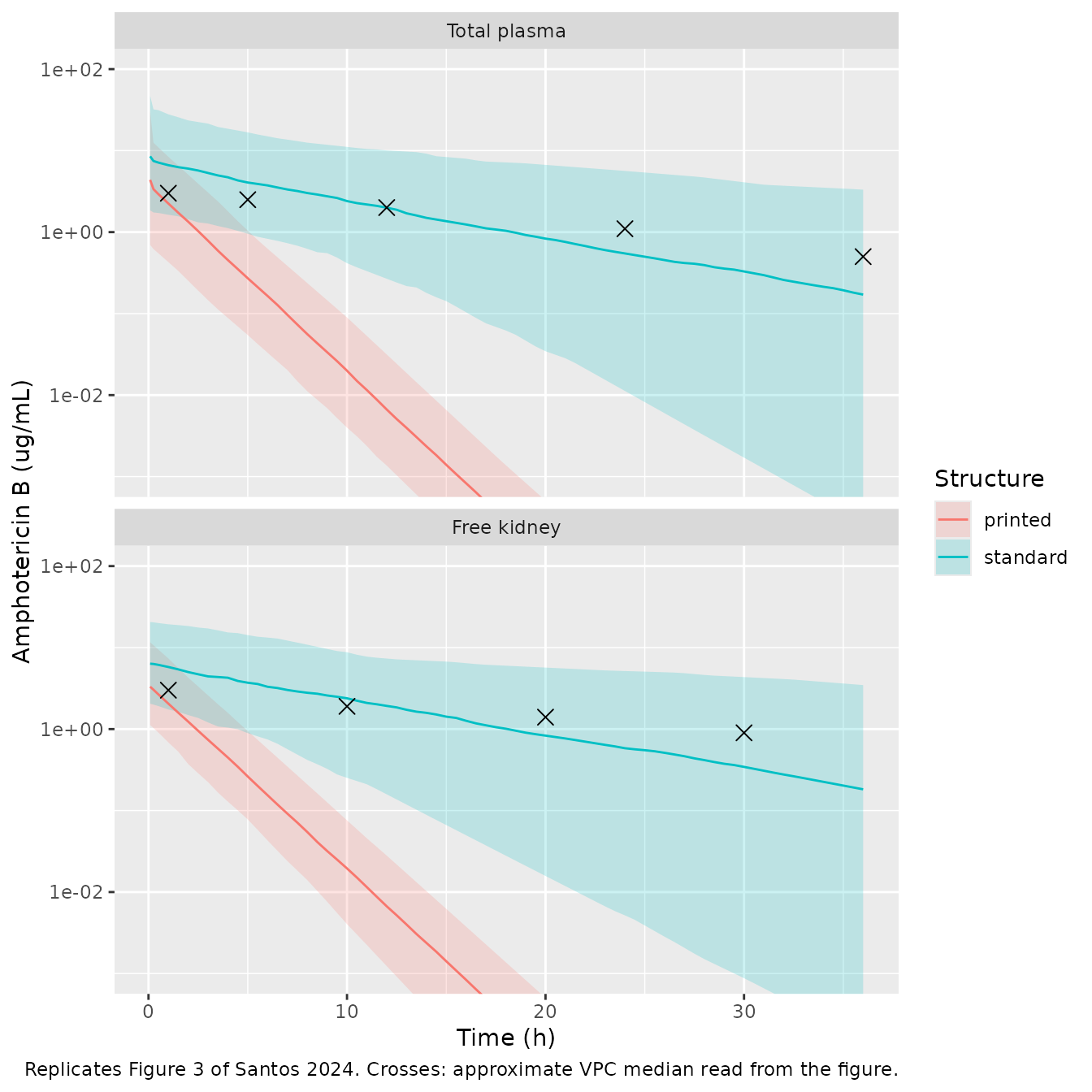
Figure 3 of Santos 2024 is a Monolix VPC. The points below are the approximate centre of its simulated-median band, read by eye from the figure by the maintainers; they are a visual guide, not digitised data. The simulated percentiles here are individual predictions without residual error, so the 5th-95th percentile band is narrower than the VPC’s (which includes the proportional residual error of 0.76 and 0.65); the median is comparable.
vpc_ref <- dplyr::bind_rows(
  data.frame(matrix = "Total plasma", time = c(1, 5, 12, 24, 36), conc = c(3, 2.5, 2, 1.1, 0.5)),
  data.frame(matrix = "Free kidney", time = c(1, 10, 20, 30), conc = c(3, 1.9, 1.4, 0.9))
)
pct <- sim |>
  dplyr::select(structure, id, time, `Total plasma` = Cc, `Free kidney` = Ckidney) |>
  tidyr::pivot_longer(c(`Total plasma`, `Free kidney`), names_to = "matrix", values_to = "conc") |>
  dplyr::filter(time > 0) |>
  dplyr::group_by(structure, matrix, time) |>
  dplyr::summarise(
    p05 = quantile(conc, 0.05), p50 = median(conc), p95 = quantile(conc, 0.95),
    .groups = "drop"
  ) |>
  dplyr::mutate(matrix = factor(matrix, levels = c("Total plasma", "Free kidney")))
vpc_ref$matrix <- factor(vpc_ref$matrix, levels = levels(pct$matrix))
ggplot(pct, aes(time, p50, colour = structure, fill = structure)) +
  geom_ribbon(aes(ymin = p05, ymax = p95), alpha = 0.2, colour = NA) +
  geom_line() +
  geom_point(data = vpc_ref, aes(time, conc), inherit.aes = FALSE, shape = 4, size = 3) +
  facet_wrap(~matrix, ncol = 1) +
  scale_y_log10() +
  coord_cartesian(ylim = c(1e-3, 100)) +
  labs(
    x = "Time (h)", y = "Amphotericin B (ug/mL)", colour = "Structure", fill = "Structure",
    caption = "Replicates Figure 3 of Santos 2024. Crosses: approximate VPC median read from the figure."
  )
med <- pct |>
  dplyr::filter(matrix == "Total plasma", time %in% c(12, 24, 36)) |>
  dplyr::select(structure, time, p50) |>
  tidyr::pivot_wider(names_from = structure, values_from = p50)
med |>
  dplyr::rename("Time (h)" = time, "Printed, median" = printed, "Standard, median" = standard) |>
knitr::kable(digits = 10, caption = "Median simulated total plasma concentration (ug/mL).")| Time (h) | Printed, median | Standard, median |
|---|---|---|
| 12 | 0.0066581625 | 1.9931446 |
| 24 | 0.0000123171 | 0.5474445 |
| 36 | 0.0000000271 | 0.1710885 |
# Orders-of-magnitude separation on cohort medians, robust to the random draw.
stopifnot(
  med$printed[med$time == 24] < 1e-3,
  med$standard[med$time == 24] > 0.2
)
The printed structure (packaged) collapses: its median plasma concentration falls below 0.01 ug/mL by 12 h and to about 1e-8 ug/mL at 36 h, whereas Figure 1 shows mean plasma concentrations near 1 ug/mL out to 36 h and the Figure 3 VPC median is about 0.5 ug/mL at 36 h. The standard structure follows the VPC median through about 12 h and then falls below it (median 0.55 ug/mL at 24 h and 0.17 ug/mL at 36 h, against roughly 1.1 and 0.5 ug/mL read from the figure), so neither structure reproduces the VPC exactly, but the standard one is far closer.
PKNCA validation
The paper computed AUC0-inf with the linear trapezoidal rule for plasma and for kidney. The same is done here on the paper’s sampling grids. The first plasma sample was drawn at 0.083 h, and the model’s bolus concentration at time zero (dose / V1, about 760 ug/mL) was never observed; trapezoiding from that value would add about 30 ugh/mL that no sampled profile contains. The plasma AUC is therefore integrated from the first sample (the 0-0.083 h slice of a sampled profile is under 0.5 ugh/mL). The kidney profile starts from its true zero at the time of dosing.
sampling <- rbind(
  data.frame(matrix = "plasma", time = setdiff(t_plasma, 0)),
  data.frame(matrix = "kidney", time = t_kidney)
)
nca_in <- sim |>
  dplyr::select(structure, id, time, plasma = Cc, kidney = Ckidney) |>
  tidyr::pivot_longer(c(plasma, kidney), names_to = "matrix", values_to = "conc") |>
  dplyr::semi_join(sampling, by = c("matrix", "time")) |>
  dplyr::filter(!is.na(conc))
dose_df <- tidyr::expand_grid(
  structure = c("printed", "standard"), matrix = c("plasma", "kidney"), id = seq_len(n_sub)
) |>
  dplyr::mutate(time = 0, amt = dose)

conc_obj <- PKNCA::PKNCAconc(nca_in, conc ~ time | structure + matrix + id)
dose_obj <- PKNCA::PKNCAdose(dose_df, amt ~ time | structure + matrix + id, route = "intravascular")
intervals <- data.frame(
  matrix = c("plasma", "kidney"), start = c(0.083, 0), end = Inf,
  aucinf.obs = TRUE, half.life = TRUE
)
nca_res <- PKNCA::pk.nca(
  PKNCA::PKNCAdata(conc_obj, dose_obj, intervals = intervals, options = list(auc.method = "linear"))
)
simulated <- as.data.frame(nca_res$result) |>
  dplyr::filter(PPTESTCD == "aucinf.obs") |>
  tidyr::crossing(rats = c("healthy", "infected"))
published <- data.frame(
  structure = rep(c("printed", "standard"), each = 4),
  matrix = rep(rep(c("plasma", "kidney"), each = 2), 2),
  rats = rep(c("healthy", "infected"), 4),
  aucinf.obs = rep(c(96.3, 59.8, 74.1, 42.3), 2)
)
cmp <- nlmixr2lib::ncaComparisonTable(
  simulated = simulated,
  reference = published,
  by = c("structure", "matrix", "rats"),
  units = c(aucinf.obs = "ug*h/mL"),
  tolerance_pct = 20
)
cmp |>
  dplyr::rename("Structure" = structure, "Matrix" = matrix, "Paper group" = rats) |>
  knitr::kable(
    digits = 1,
    caption = paste(
      "Median simulated AUC0-inf versus the paper's mean NCA AUC0-inf (Santos 2024 Results).",
      "* differs from the published value by more than 20%."
    )
)| NCA parameter | Structure | Matrix | Paper group | Reference | Simulated | % diff |
|---|---|---|---|---|---|---|
| AUC0-∞ (obs) (ug*h/mL) | printed | plasma | healthy | 96.3 | 7.52 | -92.2%* |
| AUC0-∞ (obs) (ug*h/mL) | printed | plasma | infected | 59.8 | 7.52 | -87.4%* |
| AUC0-∞ (obs) (ug*h/mL) | printed | kidney | healthy | 74.1 | 5.17 | -93.0%* |
| AUC0-∞ (obs) (ug*h/mL) | printed | kidney | infected | 42.3 | 5.17 | -87.8%* |
| AUC0-∞ (obs) (ug*h/mL) | standard | plasma | healthy | 96.3 | 81.2 | -15.7% |
| AUC0-∞ (obs) (ug*h/mL) | standard | plasma | infected | 59.8 | 81.2 | +35.7%* |
| AUC0-∞ (obs) (ug*h/mL) | standard | kidney | healthy | 74.1 | 69.4 | -6.3% |
| AUC0-∞ (obs) (ug*h/mL) | standard | kidney | infected | 42.3 | 69.4 | +64.1%* |
The packaged (printed) structure under-predicts the published plasma and kidney AUCs about 8- to 14-fold. The standard structure lies between the healthy and infected group means for both matrices; the paper’s own kidney-to-plasma AUC ratios were 0.77 (healthy) and 0.71 (infected), against 0.86 for the standard and 0.48 for the printed structure at typical values. The median simulated half-life (plasma, 0-36 h) is shown for completeness:
as.data.frame(nca_res$result) |>
  dplyr::filter(PPTESTCD == "half.life") |>
  dplyr::group_by(structure, matrix) |>
  dplyr::summarise(half_life = median(PPORRES, na.rm = TRUE), .groups = "drop") |>
  dplyr::rename("Structure" = structure, "Matrix" = matrix, "Median t1/2 (h)" = half_life) |>
knitr::kable(digits = 2)| Structure | Matrix | Median t1/2 (h) |
|---|---|---|
| printed | kidney | 1.34 |
| printed | plasma | 1.34 |
| standard | kidney | 6.82 |
| standard | plasma | 6.82 |
Assumptions and deviations
-
Equation 6 encoded as printed. The packaged model
keeps the 0.56 factor on the kidney inflow only, as published. With the
Table 1 estimates this structure loses mass (an extra elimination route
of
0.44 * k12), shortens the terminal half-life to about 1.3 h, and does not reproduce Figure 1, Figure 3 or the reported NCA AUCs. The maintainers chose the printed form so that the library reflects the publication; the standard two-compartment alternative, which reproduces the paper’s AUCs and is much closer to its VPC, is onemodel()pipe away (shown above). A third reading, applying 0.56 to both the plasma loss and the kidney gain, conserves mass and matches the plasma AUC but roughly halves kidney exposure; it is printed nowhere in the paper and is not shown. No erratum had been published as of 2026-11-09. -
IIV values read as standard deviations. Table 1
labels the IIV column “omega2”, but the accompanying CVs (106.18%,
74.71%, 58.74%, 62.34%) match
sqrt(exp(omega^2) - 1)only when the printed values are the Monolix omega SDs (0.87 gives 106%; read as a variance it would give 118%). The packaged variances are the squared values. - Residual error read as the Monolix proportional coefficient. Table 1 labels the error parameters “sigma2”; by the same reading as the IIV block, 0.76 (plasma) and 0.65 (kidney) are encoded as proportional standard deviations.
- Per-kilogram units. Volumes are reported in mL/kg, so the dose is entered in ug/kg (2.5 mg/kg = 2500 ug/kg) and concentrations come out in ug/mL. The model has no body-weight covariate.
- Kidney concentrations are free (unbound) interstitial concentrations corrected for in vivo microdialysis recovery; plasma concentrations are total. Protein binding was concentration-dependent in vitro (56.4% at 2 ug/mL, 25.5% at 8 ug/mL in healthy rat plasma) but is not part of the model.
-
Infection not retained. The C. albicans
infection covariate did not improve the fit (P > 0.05) and is
documented in
covariatesDataExcluded. - No IIV on k21, as in the paper’s final model.
- The VPC reference points in the Figure 3 replication are approximate readings of the published figure, used only as a visual guide.