Model and source
- Citation: Wu N, Katz DA, An G. A target-mediated drug disposition model to explain nonlinear pharmacokinetics of the 11beta-hydroxysteroid dehydrogenase type 1 inhibitor SPI-62 in healthy adults. J Clin Pharmacol. 2021;61(11):1442-1453. doi:10.1002/jcph.1925. PMCID:PMC8596879.
- Article: https://doi.org/10.1002/jcph.1925
- Open-access full text: https://www.ncbi.nlm.nih.gov/pmc/articles/PMC8596879/
SPI-62 is a potent, selective small-molecule inhibitor of 11-beta-hydroxysteroid dehydrogenase type 1 (HSD-1). In its phase 1 trials it showed strikingly nonlinear PK: very low plasma exposure after single low doses, a dose-dependent apparent volume, nonlinear PK after the first dose but dose-proportional PK at steady state, and accumulation ratios at low doses far larger than the elimination half-life can explain. Wu 2021 attributes all of this to target-mediated drug disposition (TMDD) – saturable, high-affinity binding of SPI-62 to a low-capacity target (taken to be HSD-1 itself) – and describes it with a two-compartment TMDD model with three transit absorption compartments.
The target binding is explicit: SPI-62 in the central compartment
binds free target with second-order rate constant Kon and
dissociates with first-order rate constant Koff. The total
number of binding sites Rtotal is constant and the
small-molecule complex is not internalised (kint = 0), so
free target is Rtotal - RC. At low doses nearly all of the
drug that reaches the central compartment is captured by the target;
once repeated dosing fills the target, the remaining disposition is
linear.
The same group later refit this structure jointly to the PK and
hepatic HSD-1 activity data (Wu_2023_SPI_62). That PK/PD
model re-estimates every PK parameter; this file is the earlier PK-only
fit and carries its own Table 2 estimates.
Units: doses must be supplied in nmol
Kon is in nM^-1 h^-1 and Rtotal is an
amount in nmol, so the model carries amounts in nmol and
Cc = central / vc is in nM. A dose in mg is converted with
the SPI-62 molecular weight. Wu 2021 does not print a molecular weight;
the value used here is 424.4 g/mol, the one implied by Wu 2023’s
conversion 0.0787 nM = 0.0334 ng/mL. It is consistent with
Wu 2021’s own statement that Rtotal = 6070 nmol
“corresponds to approximately 2.5 mg of SPI-62”.
mw_spi62 <- 424.4 # g/mol
mg_to_nmol <- function(mg) mg * 1e6 / mw_spi62
nM_to_ng_mL <- function(c_nM) c_nM * mw_spi62 / 1000

# Rtotal expressed as a mass of SPI-62 (the paper: 'approximately 2.5 mg')
round(6070 * mw_spi62 / 1e6, 2)
#> [1] 2.58
Population
Wu 2021 pooled the <= 10 mg cohorts of two phase 1 trials in healthy adults (Methods, “Data Source”, and Table 1):
- SAD/FE trial – single oral doses of 1, 3, 6 and 10 mg under fasted conditions (n = 6 active per cohort). Samples at 0.5-72 h post-dose (to 120 h for 6 mg).
- MAD trial, part B – 3 mg loading dose on day 1 then 0.2 mg once daily on days 2-14 (n = 4); 0.4 mg once daily on days 1-14 (n = 4); and 0.7 mg or 2 mg as a single dose on day 1, a 6-day washout, then once daily on days 7-20 (n = 6 each).
The analysis used 996 plasma concentrations (774 above and 222 below the LLOQ) from 44 subjects: 33 male and 11 female, mean +/- SD body weight 76.5 +/- 12.1 kg, age 20-54 years. The LLOQ was 0.1 ng/mL in the SAD/FE trial and 0.004 ng/mL in MAD part B. Age, sex, body weight and race were tested as covariates and none was retained, so the model has no covariates.
pop <- rxode2::rxode(readModelDb("Wu_2021_SPI_62"))$population
#> ℹ parameter labels from comments will be replaced by 'label()'
str(pop, max.level = 1)
#> List of 12
#>  $ species       : chr "human"
#>  $ n_subjects    : int 44
#>  $ n_studies     : int 2
#>  $ n_observations: int 996
#>  $ study_names   : chr [1:2] "SAD/FE -- SPI-62 first-in-human single-ascending-dose and food-effect trial; the fasted 1, 3, 6, and 10 mg coho"| __truncated__ "MAD part B -- SPI-62 low-dose multiple-ascending-dose cohorts (0.2, 0.4, 0.7, and 2 mg once daily)"
#>  $ age_range     : chr "20-54 years"
#>  $ weight_range  : chr "mean +/- SD 76.5 +/- 12.1 kg (range not reported)"
#>  $ sex_female_pct: num 25
#>  $ disease_state : chr "Healthy adult volunteers."
#>  $ dose_range    : chr "SAD: 1, 3, 6, and 10 mg single oral doses, fasted. MAD part B: 3 mg loading dose on day 1 then 0.2 mg once dail"| __truncated__
#>  $ regions       : chr "Not reported."
#>  $ notes         : chr "996 plasma concentrations (774 above and 222 below the LLOQ; BLQ replaced with LLOQ/2 per the Discussion). LLOQ"| __truncated__
Source trace
Every ini() value and every model()
equation, with its location in Wu 2021. The same information is an
in-file comment beside each entry of
inst/modeldb/specificDrugs/Wu_2021_SPI_62.R.
| Equation / parameter | Value | Source location |
|---|---|---|
d/dt(depot) |
n/a | Eq. 1, p. 1445 (initial condition Adepot(0) = Dose; see
Assumptions) |
d/dt(transit1) .. d/dt(transit3)
|
n/a | Eqs. 2-4, p. 1445 |
d/dt(central) |
n/a | Eq. 5, p. 1445 (transit input, kon/koff
binding, CL/Vcentral, Q exchange) |
d/dt(peripheral1) |
n/a | Eq. 6, p. 1446 |
d/dt(complex) |
n/a | Eq. 7, p. 1446
(kon * Ccentral * (Rtotal - RC) - koff * RC) |
| Exponential IIV | n/a | Eq. 8, p. 1446 |
| Proportional residual error | n/a | Eq. 9, p. 1446 |
lktr (Ktr) |
8.52 1/h | Table 2 (RSE 11%) |
lcl (CL/F) |
10.1 L/h | Table 2 (RSE 6%); apparent, Table 2 footnote a |
lvc (Vcentral/F) |
141 L | Table 2 (RSE 16%); apparent |
lq (Q/F) |
2.31 L/h | Table 2 (RSE 12%); apparent |
lvp (Vperipheral/F) |
114 L | Table 2 (RSE 7%); apparent |
lkon (Kon) |
7.1 1/(nM*h) | Table 2 (RSE 7%) |
lkoff (Koff) |
0.249 1/h | Table 2 (RSE 24%) |
lrtot (Rtotal) |
6070 nmol | Table 2 (RSE 9%) |
etalvc |
0.258394 | Table 2 IIV Vcentral 54.3% (RSE 27%, shrinkage 14%);
omega^2 = log(CV^2 + 1)
|
etalcl |
0.041560 | Table 2 IIV CL 20.6% (RSE 59%, shrinkage 22%) |
etalktr |
0.227961 | Table 2 IIV Ktr 50.6% (RSE 29%, shrinkage 8%) |
etalkoff |
0.852541 | Table 2 IIV Koff 116% (RSE 50%, shrinkage 15%) |
etalrtot |
0.120592 | Table 2 IIV Rtotal 35.8% (RSE 38%, shrinkage 12%) |
propSd |
0.268 | Table 2 proportional residual variability 26.8% (RSE 2%, shrinkage 7%) |
| MW (unit conversion only) | 424.4 g/mol | Wu 2023 conversion 0.0787 nM = 0.0334 ng/mL; see
Units |
The implied dissociation equilibrium constant cross-checks the two
binding parameters against the Discussion, which reports
Koff / Kon = 35.1 pM:
kd_nM <- 0.249 / 7.1
round(kd_nM * 1000, 1) # pM
#> [1] 35.1
Replicating Table 3 (population-predicted NCA)
Table 3 of Wu 2021 lists, next to the observed NCA values, NCA parameters computed from the population-predicted concentrations. Those are deterministic: they come from the typical-value profile at each dose, sampled at the trial’s sampling times. They are therefore the right target for an exact reproduction of the packaged parameters, with residual error and IIV removed.
mod <- readModelDb("Wu_2021_SPI_62")
mod_tv <- rxode2::zeroRe(mod)
#> ℹ parameter labels from comments will be replaced by 'label()'

# Table 1 sampling schedules
t_sad <- c(0, 0.5, 1, 1.5, 2, 3, 4, 6, 8, 10, 12, 18, 24, 36, 48, 72)
t_sad_6mg <- c(t_sad, 96, 120)
t_mad <- c(0, 0.5, 1, 1.5, 2, 3, 4, 8, 12, 16, 24)

sad_doses <- c(1, 3, 6, 10)

# One arm = one typical subject. `dose_times` in h, `obs_times` in h.
make_arm <- function(id, treatment, mg, dose_times, obs_times) {
  dplyr::bind_rows(
    data.frame(id = id, time = dose_times, evid = 1L, amt = mg_to_nmol(mg), cmt = "depot"),
    data.frame(id = id, time = obs_times, evid = 0L, amt = 0, cmt = "central")
  ) |>
    dplyr::mutate(treatment = treatment) |>
    dplyr::arrange(time, dplyr::desc(evid))
}
Single ascending doses
ev_sad <- dplyr::bind_rows(lapply(seq_along(sad_doses), function(i) {
  d <- sad_doses[i]
  make_arm(i, sprintf("%g mg", d), d, 0, if (d == 6) t_sad_6mg else t_sad)
}))

sim_sad_tv <- rxode2::rxSolve(mod_tv, ev_sad, keep = "treatment", maxsteps = 1e6) |>
  as.data.frame() |>
  dplyr::mutate(Cc = nM_to_ng_mL(Cc)) |>
  dplyr::select(id, time, Cc, treatment)
#> ℹ omega/sigma items treated as zero: 'etalvc', 'etalcl', 'etalktr', 'etalkoff', 'etalrtot'
#> Warning: multi-subject simulation without without 'omega'

# The time = 0 row is part of every schedule above (pre-dose Cc = 0).
conc_sad <- PKNCA::PKNCAconc(sim_sad_tv, Cc ~ time | treatment + id)
dose_sad <- PKNCA::PKNCAdose(
  ev_sad |> dplyr::filter(evid == 1) |> dplyr::mutate(amt = sad_doses[id]),
  amt ~ time | treatment + id
)
nca_sad <- PKNCA::pk.nca(PKNCA::PKNCAdata(
  conc_sad, dose_sad,
  intervals = data.frame(start = 0, end = Inf, cmax = TRUE, aucinf.obs = TRUE, half.life = TRUE)
))
Multiple ascending doses
Table 3 reports first-dose and last-dose NCA for the 0.4, 0.7 and 2 mg regimens. The 0.4 mg regimen is dosed on days 1-14; the 0.7 and 2 mg regimens have a single dose on day 1, a washout, and daily doses on days 7-20.
mad_regimens <- tibble::tribble(
  ~treatment, ~mg, ~last_dose,
  "0.4 mg QD", 0.4, 13 * 24,
  "0.7 mg QD", 0.7, 19 * 24,
  "2 mg QD", 2, 19 * 24
)
mad_dose_times <- function(treatment) {
  if (treatment == "0.4 mg QD") (0:13) * 24 else c(0, (6:19) * 24)
}

ev_mad <- dplyr::bind_rows(lapply(seq_len(nrow(mad_regimens)), function(i) {
  r <- mad_regimens[i, ]
  make_arm(
    i, r$treatment, r$mg, mad_dose_times(r$treatment),
    sort(unique(c(t_mad, r$last_dose + t_mad)))
  )
}))

sim_mad_tv <- rxode2::rxSolve(mod_tv, ev_mad, keep = "treatment", maxsteps = 1e6) |>
  as.data.frame() |>
  dplyr::mutate(Cc = nM_to_ng_mL(Cc)) |>
  dplyr::select(id, time, Cc, treatment)
#> ℹ omega/sigma items treated as zero: 'etalvc', 'etalcl', 'etalktr', 'etalkoff', 'etalrtot'
#> Warning: multi-subject simulation without without 'omega'

conc_mad <- PKNCA::PKNCAconc(sim_mad_tv, Cc ~ time | treatment + id)
dose_mad <- PKNCA::PKNCAdose(
  ev_mad |> dplyr::filter(evid == 1) |> dplyr::mutate(amt = mad_regimens$mg[id]),
  amt ~ time | treatment + id
)
intervals_mad <- dplyr::bind_rows(
  mad_regimens |> dplyr::transmute(treatment, start = 0, end = 24, interval = "first"),
  mad_regimens |> dplyr::transmute(treatment, start = last_dose, end = last_dose + 24, interval = "last")
) |>
  dplyr::mutate(cmax = TRUE, auclast = TRUE)
nca_mad <- PKNCA::pk.nca(PKNCA::PKNCAdata(
  conc_mad, dose_mad,
  intervals = dplyr::select(intervals_mad, -interval)
))

mad_res <- as.data.frame(nca_mad) |>
  dplyr::filter(PPTESTCD %in% c("cmax", "auclast")) |>
  dplyr::mutate(interval = ifelse(start == 0, "first", "last")) |>
  dplyr::select(treatment, interval, PPTESTCD, PPORRES) |>
  tidyr::pivot_wider(names_from = c(PPTESTCD, interval), values_from = PPORRES) |>
  dplyr::mutate(ar_cmax = cmax_last / cmax_first)
Comparison against Table 3
sim_tab <- dplyr::bind_rows(
  as.data.frame(nca_sad) |>
    dplyr::filter(PPTESTCD %in% c("cmax", "aucinf.obs", "half.life")) |>
    dplyr::transmute(treatment, parameter = PPTESTCD, simulated = PPORRES),
  mad_res |>
    tidyr::pivot_longer(-treatment, names_to = "parameter", values_to = "simulated")
)

# Wu 2021 Table 3, 'Predicted' columns
published <- tibble::tribble(
  ~treatment, ~parameter, ~published,
  "1 mg", "aucinf.obs", 57.28,
  "1 mg", "cmax", 0.05193,
  "1 mg", "half.life", 4218,
  "3 mg", "aucinf.obs", 64.45,
  "3 mg", "cmax", 2.879,
  "3 mg", "half.life", 42.99,
  "6 mg", "aucinf.obs", 362.3,
  "6 mg", "cmax", 22.42,
  "6 mg", "half.life", 54.20,
  "10 mg", "aucinf.obs", 714.8,
  "10 mg", "cmax", 48.52,
  "10 mg", "half.life", 21.95,
  "0.4 mg QD", "auclast_first", 0.07316,
  "0.4 mg QD", "auclast_last", 39.12,
  "0.4 mg QD", "cmax_first", 0.01755,
  "0.4 mg QD", "cmax_last", 3.113,
  "0.4 mg QD", "ar_cmax", 177.4,
  "0.7 mg QD", "auclast_first", 0.1472,
  "0.7 mg QD", "auclast_last", 69.42,
  "0.7 mg QD", "cmax_first", 0.03330,
  "0.7 mg QD", "cmax_last", 5.662,
  "0.7 mg QD", "ar_cmax", 170.0,
  "2 mg QD", "auclast_first", 1.246,
  "2 mg QD", "auclast_last", 198.9,
  "2 mg QD", "cmax_first", 0.1485,
  "2 mg QD", "cmax_last", 16.42,
  "2 mg QD", "ar_cmax", 110.6
)

param_labels <- c(
  cmax = "Cmax (ng/mL)",
  aucinf.obs = "AUC0-inf (ng*h/mL)",
  half.life = "t1/2 (h)",
  auclast_first = "AUC24, first dose (ng*h/mL)",
  auclast_last = "AUC24, last dose (ng*h/mL)",
  cmax_first = "Cmax, first dose (ng/mL)",
  cmax_last = "Cmax, last dose (ng/mL)",
  ar_cmax = "Accumulation ratio (Cmax)"
)

cmp <- dplyr::inner_join(published, sim_tab, by = c("treatment", "parameter")) |>
  dplyr::mutate(pct_diff = 100 * (simulated - published) / published)
stopifnot(nrow(cmp) == nrow(published))

cmp |>
  dplyr::mutate(
    parameter = param_labels[parameter],
    published = formatC(published, digits = 4, format = "fg"),
    simulated = formatC(simulated, digits = 4, format = "fg"),
    pct_diff = sprintf("%+.2f%%", pct_diff)
  ) |>
  dplyr::rename(
    "Dose" = treatment,
    "NCA parameter" = parameter,
    "Wu 2021 Table 3 (predicted)" = published,
    "This implementation" = simulated,
    "Difference" = pct_diff
  ) |>
  knitr::kable(caption = paste(
    "Typical-value NCA on the Table 1 sampling schedules versus the",
    "population-predicted column of Wu 2021 Table 3."
))| Dose | NCA parameter | Wu 2021 Table 3 (predicted) | This implementation | Difference |
|---|---|---|---|---|
| 1 mg | AUC0-inf (ng*h/mL) | 57.28 | 57.2 | -0.14% |
| 1 mg | Cmax (ng/mL) | 0.05193 | 0.05194 | +0.02% |
| 1 mg | t1/2 (h) | 4218 | 4212 | -0.14% |
| 3 mg | AUC0-inf (ng*h/mL) | 64.45 | 64.43 | -0.03% |
| 3 mg | Cmax (ng/mL) | 2.879 | 2.89 | +0.38% |
| 3 mg | t1/2 (h) | 42.99 | 42.87 | -0.29% |
| 6 mg | AUC0-inf (ng*h/mL) | 362.3 | 360.7 | -0.43% |
| 6 mg | Cmax (ng/mL) | 22.42 | 22.42 | +0.01% |
| 6 mg | t1/2 (h) | 54.2 | 54.12 | -0.15% |
| 10 mg | AUC0-inf (ng*h/mL) | 714.8 | 712 | -0.39% |
| 10 mg | Cmax (ng/mL) | 48.52 | 48.51 | -0.03% |
| 10 mg | t1/2 (h) | 21.95 | 21.93 | -0.11% |
| 0.4 mg QD | AUC24, first dose (ng*h/mL) | 0.07316 | 0.07243 | -1.00% |
| 0.4 mg QD | AUC24, last dose (ng*h/mL) | 39.12 | 39.05 | -0.17% |
| 0.4 mg QD | Cmax, first dose (ng/mL) | 0.01755 | 0.01755 | +0.02% |
| 0.4 mg QD | Cmax, last dose (ng/mL) | 3.113 | 3.118 | +0.18% |
| 0.4 mg QD | Accumulation ratio (Cmax) | 177.4 | 177.7 | +0.14% |
| 0.7 mg QD | AUC24, first dose (ng*h/mL) | 0.1472 | 0.1459 | -0.88% |
| 0.7 mg QD | AUC24, last dose (ng*h/mL) | 69.42 | 69.26 | -0.24% |
| 0.7 mg QD | Cmax, first dose (ng/mL) | 0.0333 | 0.03331 | +0.02% |
| 0.7 mg QD | Cmax, last dose (ng/mL) | 5.662 | 5.671 | +0.15% |
| 0.7 mg QD | Accumulation ratio (Cmax) | 170 | 170.3 | +0.15% |
| 2 mg QD | AUC24, first dose (ng*h/mL) | 1.246 | 1.247 | +0.07% |
| 2 mg QD | AUC24, last dose (ng*h/mL) | 198.9 | 198.3 | -0.30% |
| 2 mg QD | Cmax, first dose (ng/mL) | 0.1485 | 0.1485 | +0.01% |
| 2 mg QD | Cmax, last dose (ng/mL) | 16.42 | 16.45 | +0.16% |
| 2 mg QD | Accumulation ratio (Cmax) | 110.6 | 110.7 | +0.12% |
Every one of the 27 published predicted values is reproduced to within about 1%. Both sides are the same deterministic typical-value calculation, so the remaining differences are the rounding of Table 2 to three significant figures, the molecular weight, and the NCA software (Phoenix WinNonlin in the paper, PKNCA here), and a tight bound is appropriate:
The agreement includes the unusual single-dose values that the paper
highlights. The 1 mg AUC0-inf and 4218 h half-life look
absurd next to the 3-10 mg values, but they are what the model predicts:
over 0-72 h the 1 mg profile falls onto the target-binding plateau (see
“The terminal plateau is the binding equilibrium” below), so the last
three sampled points decline very slowly and the extrapolated tail
dominates AUC0-inf. The 2 mg first-dose Cmax
of 0.1485 ng/mL, against a last-dose Cmax of 16.4 ng/mL, is
the accumulation the paper set out to explain.
Replicating the published figures
Figure 3 – single ascending doses
t_dense <- sort(unique(c(seq(0, 24, by = 0.1), seq(24, 120, by = 1))))
ev_sad_dense <- dplyr::bind_rows(lapply(seq_along(sad_doses), function(i) {
  make_arm(i, sprintf("%g mg", sad_doses[i]), sad_doses[i], 0, t_dense)
}))
sim_sad_dense <- rxode2::rxSolve(mod_tv, ev_sad_dense, keep = "treatment", maxsteps = 1e6) |>
  as.data.frame() |>
  dplyr::mutate(
    Cc = nM_to_ng_mL(Cc),
    treatment = factor(treatment, levels = sprintf("%g mg", sad_doses))
  )
#> ℹ omega/sigma items treated as zero: 'etalvc', 'etalcl', 'etalktr', 'etalkoff', 'etalrtot'
#> Warning: multi-subject simulation without without 'omega'

ggplot(dplyr::filter(sim_sad_dense, time > 0), aes(time, Cc, colour = treatment)) +
  geom_line() +
  scale_y_log10() +
  labs(x = "Time after dose (h)", y = "SPI-62 (ng/mL)", colour = "Dose") +
  theme_bw()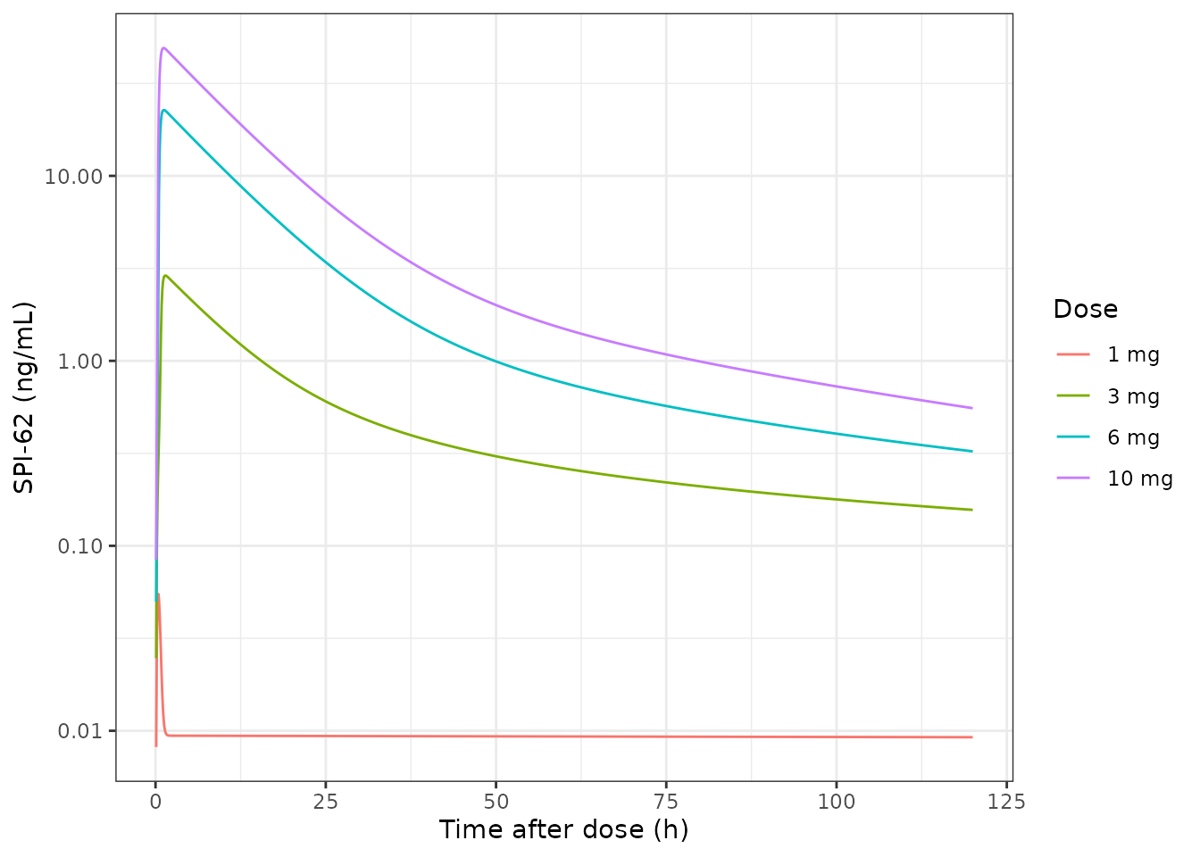
Replicates the model-predicted lines of Figure 3 of Wu 2021: typical-value SPI-62 plasma concentrations after single oral doses of 1, 3, 6 and 10 mg.
Figure 2A – dose-normalised single-dose profiles
Dose-normalised profiles superimpose only when PK is linear. The typical-value profiles are close at 6 and 10 mg and separate progressively at 3 and 1 mg, as in the paper’s Figure 2A.
sad_dn <- sim_sad_dense |>
  dplyr::mutate(dose_mg = as.numeric(sub(" mg", "", treatment)), Cc_dn = Cc / dose_mg)

ggplot(dplyr::filter(sad_dn, time > 0), aes(time, Cc_dn, colour = treatment)) +
  geom_line() +
  scale_y_log10() +
  labs(x = "Time after dose (h)", y = "SPI-62 / dose (ng/mL per mg)", colour = "Dose") +
  theme_bw()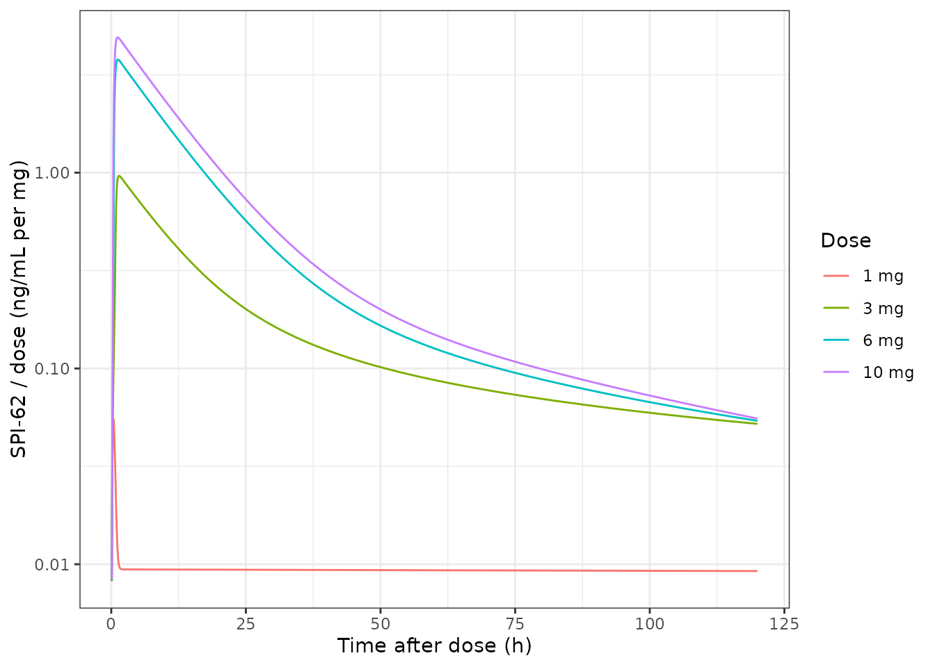
Replicates the pattern of Figure 2A of Wu 2021 using typical-value predictions: dose-normalised SPI-62 concentrations after single doses.
# Dose-normalised Cmax rises about 70-fold from 1 to 6 mg but only modestly from 6 to 10 mg.
dn_cmax <- sad_dn |>
  dplyr::group_by(treatment) |>
  dplyr::summarise(cmax_dn = max(Cc_dn), .groups = "drop")
stopifnot(
  dn_cmax$cmax_dn[dn_cmax$treatment == "6 mg"] / dn_cmax$cmax_dn[dn_cmax$treatment == "1 mg"] > 20,
  dn_cmax$cmax_dn[dn_cmax$treatment == "10 mg"] / dn_cmax$cmax_dn[dn_cmax$treatment == "6 mg"] < 1.5
)
knitr::kable(dn_cmax |> dplyr::rename("Dose" = treatment, "Cmax / dose (ng/mL per mg)" = cmax_dn), digits = 4)| Dose | Cmax / dose (ng/mL per mg) |
|---|---|
| 1 mg | 0.0549 |
| 3 mg | 0.9635 |
| 6 mg | 3.7830 |
| 10 mg | 4.9130 |
Figure 4 – multiple ascending doses
Figure 4 of Wu 2021 includes the 0.2 mg regimen (3 mg loading dose on day 1, then 0.2 mg once daily on days 2-14), which Table 3 does not tabulate.
t_mad_dense <- seq(0, 30 * 24, by = 0.5)
ev_mad_dense <- dplyr::bind_rows(
  make_arm(1, "3 mg load + 0.2 mg QD", 3, 0, t_mad_dense) |>
    dplyr::bind_rows(data.frame(
      id = 1, time = (1:13) * 24, evid = 1L, amt = mg_to_nmol(0.2),
      cmt = "depot", treatment = "3 mg load + 0.2 mg QD"
    )),
  make_arm(2, "0.4 mg QD", 0.4, mad_dose_times("0.4 mg QD"), t_mad_dense),
  make_arm(3, "0.7 mg QD", 0.7, mad_dose_times("0.7 mg QD"), t_mad_dense),
  make_arm(4, "2 mg QD", 2, mad_dose_times("2 mg QD"), t_mad_dense)
) |>
  dplyr::arrange(id, time, dplyr::desc(evid))

sim_mad_dense <- rxode2::rxSolve(mod_tv, ev_mad_dense, keep = "treatment", maxsteps = 1e6) |>
  as.data.frame() |>
  dplyr::mutate(Cc = nM_to_ng_mL(Cc))
#> ℹ omega/sigma items treated as zero: 'etalvc', 'etalcl', 'etalktr', 'etalkoff', 'etalrtot'
#> Warning: multi-subject simulation without without 'omega'

ggplot(dplyr::filter(sim_mad_dense, time > 0), aes(time / 24, Cc)) +
  geom_line() +
  facet_wrap(~treatment) +
  scale_y_log10() +
  labs(x = "Time after first dose (days)", y = "SPI-62 (ng/mL)") +
  theme_bw()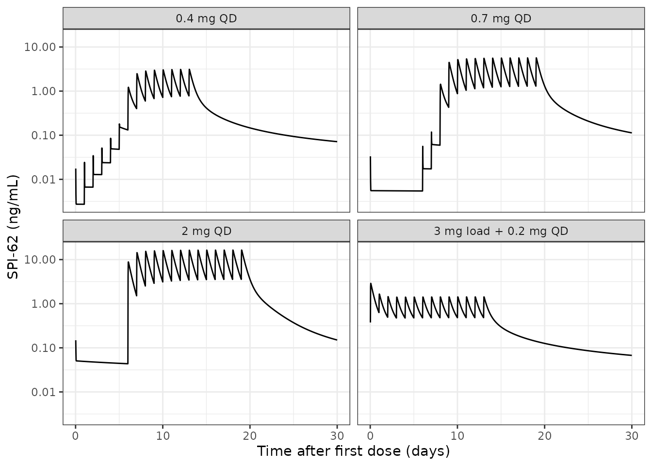
Replicates the model-predicted lines of Figure 4 of Wu 2021: typical-value SPI-62 plasma concentrations for the four MAD part B regimens.
The terminal plateau is the binding equilibrium
After a low dose the free SPI-62 concentration becomes pinned to the
binding equilibrium with the (mostly occupied) target,
C = Kd * RC / (Rtotal - RC), and drains only as fast as the
complex releases drug. That is why the 1 mg typical-value profile is
almost flat in its terminal phase and why Table 3’s 1 mg half-life is
4218 h. The simulated concentration agrees with the equilibrium
expression evaluated from the simulated complex amount:
sim_1mg <- rxode2::rxSolve(
  mod_tv,
  make_arm(1, "1 mg", 1, 0, c(0, 24, 48, 72, 120, 240, 480)),
  maxsteps = 1e6
) |>
  as.data.frame() |>
  dplyr::filter(time >= 24) |>
  dplyr::mutate(
    C_equilibrium = kd_nM * complex / (6070 - complex),
    ratio = Cc / C_equilibrium,
    Cc_ng_mL = nM_to_ng_mL(Cc)
  )
#> ℹ omega/sigma items treated as zero: 'etalvc', 'etalcl', 'etalktr', 'etalkoff', 'etalrtot'

knitr::kable(
  sim_1mg |>
    dplyr::select(time, Cc_ng_mL, complex, ratio) |>
    dplyr::rename(
      "Time (h)" = time,
      "Cc (ng/mL)" = Cc_ng_mL,
      "Complex (nmol)" = complex,
      "Cc / equilibrium C" = ratio
    ),
  digits = 4
)| Time (h) | Cc (ng/mL) | Complex (nmol) | Cc / equilibrium C |
|---|---|---|---|
| 24 | 0.0094 | 2346.158 | 0.9996 |
| 48 | 0.0093 | 2340.266 | 0.9996 |
| 72 | 0.0093 | 2334.616 | 0.9996 |
| 120 | 0.0092 | 2323.728 | 0.9996 |
| 240 | 0.0091 | 2297.522 | 0.9996 |
| 480 | 0.0087 | 2246.857 | 0.9996 |
Stochastic simulation and PKNCA
A virtual cohort of 100 subjects per SAD dose shows the between-subject variability the model carries. The model has no covariates, so no covariate distribution is needed.
rxode2::rxSetSeed(20211101)
n_per_arm <- 100
ev_vpc <- dplyr::bind_rows(lapply(seq_along(sad_doses), function(i) {
  dplyr::bind_rows(lapply(seq_len(n_per_arm), function(j) {
    make_arm((i - 1) * n_per_arm + j, sprintf("%g mg", sad_doses[i]), sad_doses[i], 0, t_sad)
  }))
}))

sim_vpc <- rxode2::rxSolve(mod, ev_vpc, keep = "treatment", maxsteps = 1e6) |>
  as.data.frame() |>
  dplyr::mutate(
    Cc = nM_to_ng_mL(Cc),
    treatment = factor(treatment, levels = sprintf("%g mg", sad_doses))
  )
#> ℹ parameter labels from comments will be replaced by 'label()'
vpc_sum <- sim_vpc |>
  dplyr::filter(time > 0) |>
  dplyr::group_by(treatment, time) |>
  dplyr::summarise(
    p05 = quantile(sim, 0.05), p50 = median(sim), p95 = quantile(sim, 0.95),
    .groups = "drop"
  ) |>
  dplyr::mutate(dplyr::across(c(p05, p50, p95), nM_to_ng_mL))

ggplot(vpc_sum, aes(time)) +
  geom_ribbon(aes(ymin = p05, ymax = p95), alpha = 0.3) +
  geom_line(aes(y = p50)) +
  facet_wrap(~treatment, scales = "free_y") +
  scale_y_log10() +
  labs(x = "Time after dose (h)", y = "SPI-62 (ng/mL)") +
  theme_bw()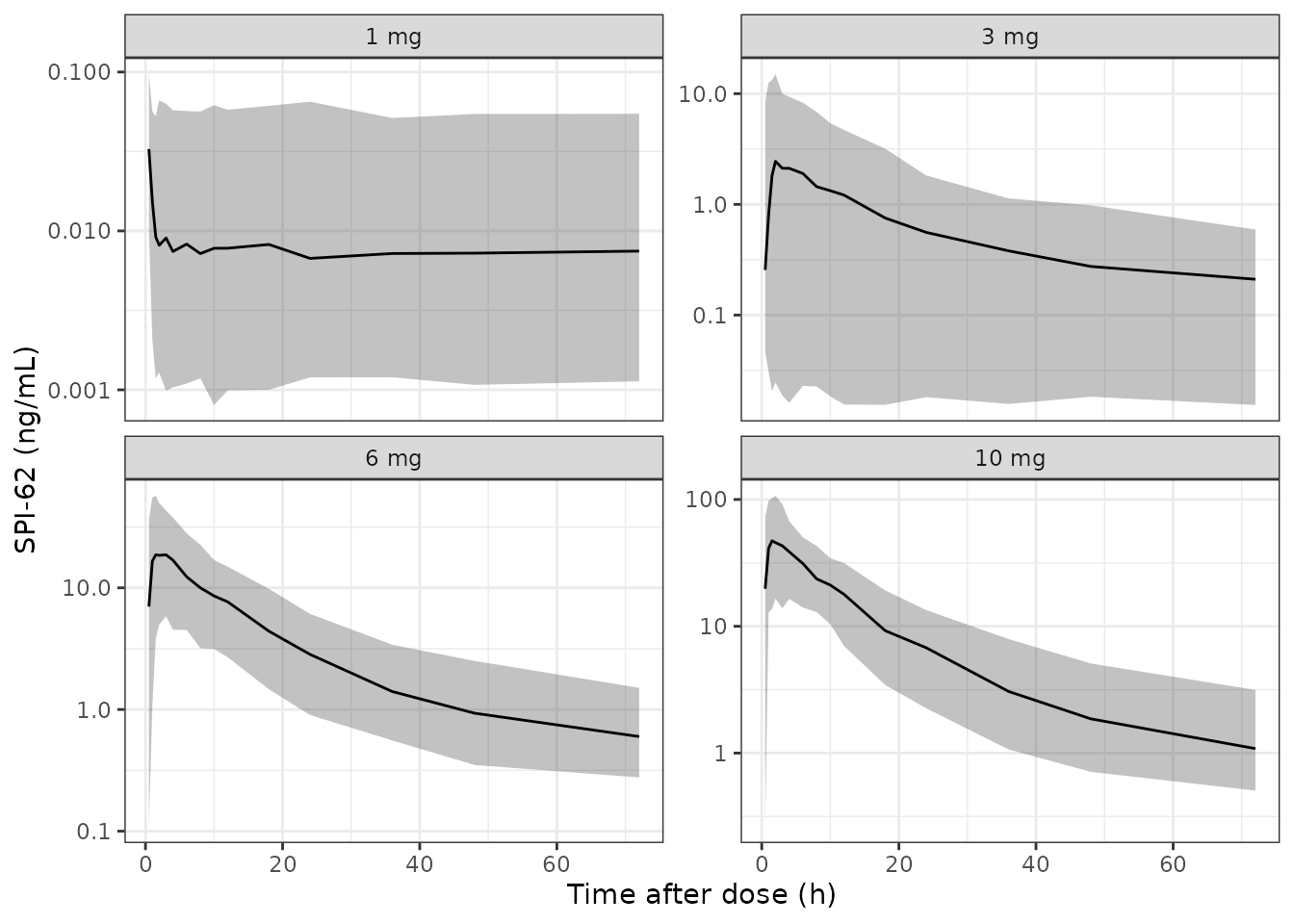
Median and 5th-95th percentile of simulated SPI-62 concentrations (with residual error), 100 virtual subjects per single dose, on the Table 1 SAD sampling schedule.
NCA on the simulated individual profiles (without residual error, i.e. the individual predictions) over the SAD sampling schedule:
nca_in <- sim_vpc |>
  dplyr::filter(!is.na(Cc)) |>
  dplyr::select(id, time, Cc, treatment)

conc_obj <- PKNCA::PKNCAconc(nca_in, Cc ~ time | treatment + id)
dose_obj <- PKNCA::PKNCAdose(
  ev_vpc |>
    dplyr::filter(evid == 1) |>
    dplyr::mutate(amt = as.numeric(sub(" mg", "", treatment))) |>
    dplyr::select(id, time, amt, treatment),
  amt ~ time | treatment + id
)
nca_vpc <- PKNCA::pk.nca(PKNCA::PKNCAdata(
  conc_obj, dose_obj,
  intervals = data.frame(start = 0, end = 72, cmax = TRUE, tmax = TRUE, auclast = TRUE)
))

nca_vpc_sum <- as.data.frame(nca_vpc) |>
  dplyr::filter(PPTESTCD %in% c("cmax", "tmax", "auclast")) |>
  dplyr::mutate(treatment = factor(treatment, levels = sprintf("%g mg", sad_doses))) |>
  dplyr::group_by(treatment, PPTESTCD) |>
  dplyr::summarise(
    median = median(PPORRES, na.rm = TRUE),
    p05 = quantile(PPORRES, 0.05, na.rm = TRUE),
    p95 = quantile(PPORRES, 0.95, na.rm = TRUE),
    .groups = "drop"
  )

nca_vpc_sum |>
  dplyr::mutate(
    PPTESTCD = dplyr::recode(PPTESTCD, cmax = "Cmax (ng/mL)", tmax = "Tmax (h)", auclast = "AUC0-72 (ng*h/mL)"),
    value = sprintf("%s (%s - %s)", signif(median, 3), signif(p05, 3), signif(p95, 3))
  ) |>
  dplyr::select(treatment, PPTESTCD, value) |>
  dplyr::rename("Dose" = treatment, "NCA parameter" = PPTESTCD, "Median (5th-95th percentile)" = value) |>
knitr::kable(caption = "Simulated single-dose NCA, 100 virtual subjects per dose.")| Dose | NCA parameter | Median (5th-95th percentile) |
|---|---|---|
| 1 mg | AUC0-72 (ng*h/mL) | 0.584 (0.0947 - 4.06) |
| 1 mg | Cmax (ng/mL) | 0.0394 (0.0145 - 0.0967) |
| 1 mg | Tmax (h) | 0.5 (0.5 - 1) |
| 3 mg | AUC0-72 (ng*h/mL) | 58.6 (1.37 - 162) |
| 3 mg | Cmax (ng/mL) | 2.62 (0.0738 - 13.9) |
| 3 mg | Tmax (h) | 1.5 (0.5 - 3) |
| 6 mg | AUC0-72 (ng*h/mL) | 290 (122 - 506) |
| 6 mg | Cmax (ng/mL) | 21.6 (6.5 - 55.1) |
| 6 mg | Tmax (h) | 1.5 (0.5 - 3) |
| 10 mg | AUC0-72 (ng*h/mL) | 638 (410 - 909) |
| 10 mg | Cmax (ng/mL) | 50.7 (20 - 102) |
| 10 mg | Tmax (h) | 1.5 (0.5 - 2) |
For context, Table 3 also reports the observed
geometric-mean Cmax: 0.1296, 1.903, 25.65 and 62.63 ng/mL
at 1, 3, 6 and 10 mg (CV 156%, 110%, 40% and 24%). The simulated medians
sit near the observed values at 3-10 mg. At 1 mg the observed mean is
higher than the model’s typical value (0.052 ng/mL); most 1 mg samples
were below the 0.1 ng/mL LLOQ and were imputed as LLOQ/2 in the fit,
which the paper notes is where the model fit is weakest.
# Centre of the simulated Cmax distribution at 6 and 10 mg against the observed
# geometric means (Table 3); both are well-quantified doses.
sim_cmax <- nca_vpc_sum |> dplyr::filter(PPTESTCD == "cmax")
obs_cmax <- c(`6 mg` = 25.65, `10 mg` = 62.63)
ratio_cmax <- sim_cmax$median[match(names(obs_cmax), as.character(sim_cmax$treatment))] / obs_cmax
ratio_cmax
#>      6 mg     10 mg
#> 0.8419691 0.8093500
stopifnot(all(ratio_cmax > 0.6 & ratio_cmax < 1.4))
Assumptions and deviations
-
Eq. 1 is printed as
dAdepot/dt = -ktr * Dose. Taken literally the depot would lose drug at a constant rate forever. The depot amountAdepotis used instead: that is the standard first-order form, the only one consistent with Eq. 2 (which takesktr * Adepotas the input to the first transit compartment), and the form the same authors print in Wu 2023. The exact reproduction of Table 3 above confirms it. - Molecular weight is not printed in Wu 2021. 424.4 g/mol is the value implied by Wu 2023 for the same compound and is consistent with Wu 2021’s “6070 nmol corresponds to approximately 2.5 mg” (2.58 mg at 424.4 g/mol). It affects only the mg-to-nmol dose conversion and the nM-to-ng/mL output conversion, not any estimated parameter; the Table 3 reproduction to within about 1% is consistent with it.
-
No bioavailability term. Wu 2021 writes the depot
initial condition as
Dose(no F) and Table 2 footnote a states that volumes and clearances are apparent because F is unknown. The model therefore has nof(depot), and all volumes and flows are apparent (per unit F). -
IIV percentages are treated as coefficients of
variation. Table 2 reports each IIV as a percentage for an
exponential IIV model (Eq. 8); the internal variances use
omega^2 = log(CV^2 + 1). The paper does not say whether the percentages are exact CVs orsqrt(omega^2) * 100; the two readings differ materially only forKoff(116%:omega^20.853 versus 1.346). The typical-value replication above does not depend on this choice. -
Residual error is read as an SD. Table 2 labels the
residual term
sigma^2with unit “%” and value 26.8%. It is encoded as a proportional SD of 0.268 (a 26.8% CV), the conventional reading of a percentage and the one used for the same quantity in Wu 2023. - No off-diagonal IIV. Table 2 reports five variances and no covariances.
- Accumulation-ratio typo in the text. The Results text gives the predicted 0.4 mg accumulation ratio as 117.4, while Table 3 gives 177.4. Table 3 is internally consistent (3.113 / 0.01755 = 177.4) and is the value used above.
-
Covariates. Age, sex, body weight and race were
tested and not retained; they are documented in
covariatesDataExcluded. Wu 2021 does not report the race composition. - Virtual cohort size. The paper’s Appendix 1 simulated 200 replicates of each subject; the stochastic section here uses 100 virtual subjects per dose to stay inside the vignette render budget. The Table 3 reproduction does not use the stochastic cohort.