RNA lipid nanoparticle disposition and cellular transport (Wang 2024)
Source:vignettes/articles/Wang_2024_rnaLipidNanoparticle.Rmd
Wang_2024_rnaLipidNanoparticle.RmdModel and source
Wang 2024 builds a multi-scale model of RNA lipid-nanoparticle (LNP) delivery: three semi-mechanistic whole-body PBPK models for the in vivo disposition of the ionizable lipid in rats, mice and humans, and a cellular PBPK model of LNP trafficking inside HeLa cells. A quantum-mechanics calculation of ionizable-lipid biodegradability accompanies them; that part is not an ODE model and is summarised here without being packaged.
The paper contributes four models to nlmixr2lib:
| Model | Scale | Formulations covered |
|---|---|---|
Wang_2024_ionizableLipid_rat_pbpk |
rat whole body | MC3, SM-102, Lipid 5 |
Wang_2024_ionizableLipid_mouse_pbpk |
mouse whole body | MC3 80 nm, DMAP-BLP 78 nm, DMAP-BLP 45 nm |
Wang_2024_patisiran_human_pbpk |
human whole body | patisiran (MC3) |
Wang_2024_ionizableLipid_hela_qsp |
HeLa cell | C12-200, MC3, L319 |
- Citation: Wang W, Deng S, Lin J, Ouyang D (2024). Modeling on in vivo disposition and cellular transportation of RNA lipid nanoparticles via quantum mechanics/physiologically-based pharmacokinetic approaches. Acta Pharm Sin B 14(10):4591-4607. doi:10.1016/j.apsb.2024.06.011. Model equations Eqs. (1)-(9) and the full SimBiology ODE export in the Supporting Information (mmc1.pdf) section 1; physiology from Table 1 (‘Rat’ column); fitted parameters from Figure 4A.
- Article: https://doi.org/10.1016/j.apsb.2024.06.011
- Supplement (full SimBiology ODE export, Figures S1-S7, Table S1): https://doi.org/10.1016/j.apsb.2024.06.011 (Appendix A,
mmc1.pdf)
mod_rat   <- readModelDb("Wang_2024_ionizableLipid_rat_pbpk")
mod_mouse <- readModelDb("Wang_2024_ionizableLipid_mouse_pbpk")
mod_human <- readModelDb("Wang_2024_patisiran_human_pbpk")
mod_cell  <- readModelDb("Wang_2024_ionizableLipid_hela_qsp")
Population
The three in vivo models were fitted to pooled mean concentration-time profiles digitised from previously published studies, not to individual-subject data, so none of them carries between-subject variability.
-
Rat
(
Wang_2024_ionizableLipid_rat_pbpk) - Sprague-Dawley rats, 225-250 g (0.2375 kg reference body weight, Table 1), given a single intravenous hEPO-mRNA-LNP dose of 0.2 mg/kg mRNA. The LNP was ionizable lipid : DSPC : cholesterol : PEG-lipid at 50:10:38.5:1.5 molar ratio with an estimated N/P ratio of 5.67. Liver and spleen ionizable-lipid concentrations were followed for 48 h for three ionizable lipids (MC3, SM-102, Lipid 5). -
Mouse
(
Wang_2024_ionizableLipid_mouse_pbpk) - two studies. CD-1 mice, 6-8 weeks, given FVII-siRNA-LNP built on MC3 at 0.33, 3.3 and 11.1 mg/kg lipid (exposure was dose-linear, so only the 11.1 mg/kg arm was fitted); and C57BL/6 mice, 6-8 weeks, given 0.3 mg/kg FVII siRNA (about 3.42 mg/kg ionizable lipid) as DMAP-BLP LNP at 78 nm and 45 nm. Reference body weight 0.0270 kg. Both studies traced the particle with 3H-CHE, a non-exchangeable, non-metabolisable lipid label. -
Human (
Wang_2024_patisiran_human_pbpk) - healthy volunteers in the patisiran (Onpattro) phase 1 trials ALN-TTR02-001 and ALN-TTR02-005, dosed intravenously at 0.01, 0.05, 0.15, 0.3 and 0.5 mg/kg siRNA. Reference body weight 69.70 kg (Table 1). Plasma MC3 was followed for more than 4000 h. -
HeLa cells
(
Wang_2024_ionizableLipid_hela_qsp) - confocal and electron microscopy time courses of LNP uptake, vesicle co-localisation and siRNA release from three published HeLa studies covering C12-200, MC3 and L319.
The same information is available programmatically, e.g.
readModelDb("Wang_2024_ionizableLipid_rat_pbpk")()$population.
Model structure
All three in vivo models share one skeleton (paper Figure
2): a venous pool, an arterial pool, a lung blood vessel that is a pure
pass-through, and three organ groups - liver, spleen and a lumped “other
organs” compartment. Liver and spleen are each resolved into a vascular
space, an interstitium and an intracellular space. LNP crosses the
sinusoidal endothelium by passive permeation (P x S, Eq.
3), is internalised by receptor-mediated uptake whose rate is
proportional to an LDL-receptor concentration (Eq. 4), disassembles to
release free ionizable lipid (Eq. 5), and the free lipid is hydrolysed
by esterase (Eq. 6). The species differences are which of those routes
is switched on:
| Route | Rat | Mouse | Human |
|---|---|---|---|
| Permeation into liver | on | on | on |
| Permeation into spleen | on | on | off |
LNP disassembly (kdis) in liver / spleen |
on | off | off |
Free-lipid hydrolysis (kel) in liver / spleen |
on | off | off |
| Elimination in “other organs” | on | on | off |
LNP dissociation in blood / interstitium (kf) |
off | on | off |
The cellular model (paper Figure 3, right panel) is a linear
trafficking chain: early endosome to late endosome to lysosome, with the
late endosome additionally egressing material out of the cell
(keg) and undergoing an endosomal-escape event
(krel) that sends a fraction frel of its siRNA
into the cytoplasm and the remainder, plus all the lipid, into an
autophagosome that matures into an autolysosome.
Source trace
Every ini() entry carries an in-file comment naming its
source location. The table below collects them. Values in Figures 4A,
5A-5C, 6A, 7, 8C and 9D are in parameter tables that are part of the
figure images rather than the article text layer, so they cannot be
found by a text search of the PDF; they were read from the published
figure panels.
| Model | Equation / parameter | Value | Source location |
|---|---|---|---|
| all in vivo | organ volumes, blood flows, endothelium surface areas, hematocrit | see model()
|
Table 1 |
| all in vivo |
dM/dt artery to organ blood, organ blood to vein |
n/a | Eqs. (1), (2) |
| all in vivo | dM/dt = P * S * (Cblood - Cinter) |
n/a | Eq. (3) |
| all in vivo | dM/dt = kin * Cinter * Creceptor * Vinter |
n/a | Eq. (4) |
| rat | dM/dt = kdis * Ccell * Vcell |
n/a | Eq. (5) |
| rat | dM/dt = kel * Ccell * Vcell |
n/a | Eq. (6) |
| rat | X = X_MC3 * Scale_X |
n/a | Eq. (8) |
| all in vivo | Creceptor,spleen = Creceptor,liver * Scale_receptor |
n/a | Eq. (9) |
| all in vivo | full compartmental ODE set | n/a | Supporting Information sections 1.2 and 2.2 |
| all in vivo | whole-organ and blood observation formulas | n/a | Supporting Information sections 1.1 and 2.1 |
| rat |
lp_liver_mc3, lp_liver_lipid5
|
2.6112, 0.5222 | Figure 4A, “P to liver” |
| rat | lp_spleen_* |
0.0026, 0.0020, 5.0e-4 | Figure 4A, “P to spleen” |
| rat | lp_other_* |
0.0135, 2.1e-5, 0.0020 | Figure 4A, “P to other” |
| rat |
lkel_liver, lkel_spleen
|
3.7943, 0.0627 | Figure 4A, “kel in liver / spleen” |
| rat | lkel_other_* |
0.0143, 0.0200, 0.0495 | Figure 4A, “kel in other” |
| rat |
lkin, lkdis
|
20.0013, 0.0193 | Figure 4A, “kin”, “kdis” |
| rat |
lscale_kin_*, lscale_kdis_*,
lscale_kel_*
|
see file | Figure 4A, “Scale of …” |
| rat, mouse | creceptor_liver |
1.000 | Table 1, footnote b (assumed) |
| rat, mouse | lscale_receptor |
0.3729, 0.1217 | Table 1, “Receptor scaling from the liver to spleen” |
| mouse |
lp_liver_*, lp_spleen_*,
lp_other_*
|
see file | Figures 5A, 5B, 5C |
| mouse |
lkel_other_*, lkin_*
|
see file | Figures 5A, 5B, 5C |
| mouse |
lkf_dmap78, lkf_dmap45
|
0.0414, 0.1089 | Figure 6A |
| human |
lp_liver, lp_other, lkin
|
5.7e-4, 3.6e-5, 10.8241 | Figure 7 |
| human |
p_spleen, kel_other switched off |
0 | Section 3.1.4 |
| cell | trafficking chain dM/dt
|
n/a | Eqs. (10)-(17); Supporting Information section 4.2 |
| cell |
lkee_le, lkle_ly, lkeg
|
3.3820, 0.2094, 0.5222 | Figure 8C, “Reduced model” column |
| cell |
lkrel_c12200, lkrel_mc3,
lkrel_l319
|
0.0080, 0.0058, 0.0157 | Figures 8C and 9D |
| cell | frel |
0.5 | Figure 9D; section 3.2.2 |
| cell | kAP_AL = kLE_LY |
n/a | Section 2.2.2 |
| cell | no metabolism of lipid or RNA | n/a | Table S1, assumption 5 |
Dose conversion
The models track the ionizable lipid, but the studies report RNA doses. The paper supplies the conversion for two of the three species, and both give essentially the same lipid-per-RNA mass ratio.
dose_conv <- tibble::tribble(
  ~Species, ~`RNA dose (mg/kg)`, ~`Lipid dose (mg/kg)`, ~`mg lipid per mg RNA`, ~Source,
  "Rat (MC3)",            0.2,  2.23, 2.23 / 0.2,  "Figure 4A legend",
  "Rat (SM-102, Lipid 5)", 0.2,  2.46, 2.46 / 0.2,  "Figure 4A legend",
  "Mouse (DMAP-BLP)",     0.3,  3.42, 3.42 / 0.3,  "Section 3.1.3"
)
knitr::kable(dose_conv, digits = 2,
caption = "Ionizable-lipid dose per unit RNA dose, as reported by Wang 2024.")| Species | RNA dose (mg/kg) | Lipid dose (mg/kg) | mg lipid per mg RNA | Source |
|---|---|---|---|---|
| Rat (MC3) | 0.2 | 2.23 | 11.15 | Figure 4A legend |
| Rat (SM-102, Lipid 5) | 0.2 | 2.46 | 12.30 | Figure 4A legend |
| Mouse (DMAP-BLP) | 0.3 | 3.42 | 11.40 | Section 3.1.3 |
Wang 2024 does not state the MC3 mass corresponding to a patisiran dose, but section 2.1.1 records that the patisiran LNP formulation “is very similar to that in the above mouse study”. The MC3-specific ratio of 11.15 mg lipid per mg RNA from the rat legend is therefore used for the human simulations below, and the resulting initial plasma concentration is checked against Figure 7.
mg_mc3_per_mg_rna <- 2.23 / 0.2   # 11.15, Figure 4A legend

bw_rat   <- 0.2375  # kg, Table 1
bw_mouse <- 0.0270  # kg, Table 1
bw_human <- 69.70   # kg, Table 1

dose_rat_mc3   <- 2.23 * bw_rat
dose_rat_other <- 2.46 * bw_rat
dose_mouse_mc3 <- 11.1 * bw_mouse
dose_mouse_dmap <- 3.42 * bw_mouse
Rat: three ionizable lipids (Figure 4A)
rat_arm <- function(label, sm102, lipid5, dose) {
  ev <- rxode2::et(amt = dose, cmt = "venous_np") |>
    rxode2::et(seq(0, 48, by = 0.25), cmt = "venous_np")
  as.data.frame(ev) |>
    dplyr::mutate(id = 1L, lipid = label,
                  FORM_LNP_SM102 = sm102, FORM_LNP_LIPID5 = lipid5)
}

rat_events <- dplyr::bind_rows(
  rat_arm("MC3",     0L, 0L, dose_rat_mc3),
  rat_arm("SM-102",  1L, 0L, dose_rat_other),
  rat_arm("Lipid 5", 0L, 1L, dose_rat_other)
)

rat_sim <- rat_events |>
  dplyr::group_split(lipid) |>
  lapply(function(d) {
    rxode2::rxSolve(mod_rat, d, keep = "lipid", useLinCmt = FALSE) |>
      as.data.frame()
  }) |>
  dplyr::bind_rows()
# Replicates Figure 4A of Wang 2024: liver and spleen ionizable-lipid
# concentration after a single IV mRNA-LNP dose in rats.
rat_sim |>
  dplyr::select(time, lipid, Liver = Cliver, Spleen = Cspleen) |>
  tidyr::pivot_longer(c(Liver, Spleen), names_to = "Organ", values_to = "conc") |>
  ggplot(aes(time, conc, colour = Organ)) +
  geom_line(linewidth = 0.8) +
  facet_wrap(~lipid, scales = "free_y") +
  labs(x = "Time (h)", y = "Lipid concentration (mg/mL)",
       title = "Figure 4A - rat liver and spleen ionizable lipid",
       caption = "Replicates Figure 4A of Wang 2024.") +
  theme_bw()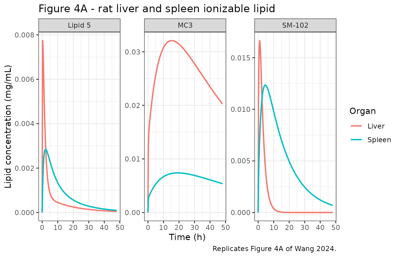
The paper plots no numeric table for these curves, so the comparison below uses landmark values read from the Figure 4A panels.
rat_landmarks <- rat_sim |>
  dplyr::group_by(lipid) |>
  dplyr::summarise(
    `Liver peak (mg/mL)` = max(Cliver),
    `Liver Tmax (h)`     = time[which.max(Cliver)],
    `Spleen peak (mg/mL)` = max(Cspleen),
    .groups = "drop"
  )

rat_published <- tibble::tribble(
  ~lipid,    ~`Liver peak, Fig 4A`, ~`Liver Tmax, Fig 4A`, ~`Spleen peak, Fig 4A`,
  "MC3",     0.037,  15, 0.020,
  "SM-102",  0.017,   1, 0.020,
  "Lipid 5", 0.0060,  1, 0.0035
)

rat_landmarks |>
  dplyr::left_join(rat_published, by = "lipid") |>
  dplyr::relocate(lipid) |>
  knitr::kable(digits = 4,
               caption = paste("Rat landmark comparison. Published values are",
                               "read from the Figure 4A panels and are",
"approximate."))| lipid | Liver peak (mg/mL) | Liver Tmax (h) | Spleen peak (mg/mL) | Liver peak, Fig 4A | Liver Tmax, Fig 4A | Spleen peak, Fig 4A |
|---|---|---|---|---|---|---|
| Lipid 5 | 0.0077 | 0.25 | 0.0028 | 0.006 | 1 | 0.0035 |
| MC3 | 0.0321 | 15.25 | 0.0074 | 0.037 | 15 | 0.0200 |
| SM-102 | 0.0167 | 1.00 | 0.0124 | 0.017 | 1 | 0.0200 |
The liver curve is reproduced closely for all three lipids in both magnitude and shape: the MC3 peak time is exact (15.2 h simulated vs about 15 h published) and the SM-102 peak is within 2%. The spleen curves are systematically low; the mouse section below shows that this is a property of the published parameter set rather than of the transcription, and the Errata quantifies it.
A second, parameter-free check on the rat model is the ratio of the
liver and spleen uptake clearances,
kin x Creceptor x Vinterstitium, which sets the long-run
split of the dose between the two organs:
rat_ratio <- tibble::tibble(
  Quantity = c("Liver uptake clearance (mL/h)",
               "Spleen uptake clearance (mL/h)",
               "Liver : spleen ratio",
               "Liver : spleen organ mass ratio at 48 h, Figure 4A"),
  Value = c(20.0013 * 1 * 1.718,
            20.0013 * 0.3729 * 0.09390,
            (20.0013 * 1 * 1.718) / (20.0013 * 0.3729 * 0.09390),
            (0.024 * 10.74) / (0.011 * 0.4507))
)
knitr::kable(rat_ratio, digits = 2,
caption = "Rat organ-uptake split implied by the published parameters.")| Quantity | Value |
|---|---|
| Liver uptake clearance (mL/h) | 34.36 |
| Spleen uptake clearance (mL/h) | 0.70 |
| Liver : spleen ratio | 49.06 |
| Liver : spleen organ mass ratio at 48 h, Figure 4A | 51.99 |
The model’s 49.1 and the figure’s 52.0 agree to 6%, which confirms
both the direction of the Eq. (9) receptor scaling and the
interpretation of the P x S permeation term discussed
next.
The P x S unit convention
Wang 2024 tabulates the permeability P in cm/s and the
endothelium surface area S in cm^2, so P x S
is nominally cm^3/s and would need a factor of 3600 to become the mL/h
coefficient the rest of the model works in. The models here use
P x S directly on the mL/h scale, without that
factor. Two independent lines of evidence settle this.
First, the paper’s own parameter-sensitivity analysis. Figure S4’s
caption and section 3.1.2 state that permeability “shows a minimal
influence on the liver PK profile, but the spleen PK profile is very
sensitive to the change of permeability”. Without the 3600 factor, the
rat liver P x S is 3062 mL/h against a 737 mL/h hepatic
blood flow (perfusion-limited, so insensitive to P) while
the spleen is 0.44 mL/h against a 39.6 mL/h splenic flow
(permeability-limited, so highly sensitive). With the factor, both
organs would be strongly perfusion-limited and neither would be
sensitive to P.
Second, the fit itself. Rat MC3 is insensitive to the choice - which is exactly what the sensitivity analysis predicts for a perfusion-limited liver - but every other liver curve collapses under the 3600 factor:
ps_arms <- tibble::tribble(
  ~lipid,    ~sm102, ~lipid5, ~dose,           ~p_liver, ~p_spleen, ~p_other, ~published,
  "MC3",     0L,     0L,      dose_rat_mc3,    2.6112,   0.0026,    0.0135,   0.037,
  "SM-102",  1L,     0L,      dose_rat_other,  2.6112,   0.0020,    2.1e-5,   0.017,
  "Lipid 5", 0L,     1L,      dose_rat_other,  0.5222,   5.0e-4,    0.0020,   0.0060
)

ps_scan <- lapply(seq_len(nrow(ps_arms)), function(i) {
  a <- ps_arms[i, ]
  peaks <- vapply(c(1, 3600), function(sc) {
    d <- rat_arm(a$lipid, a$sm102, a$lipid5, a$dose)
    p <- c(lp_liver_mc3 = log(2.6112 * sc), lp_liver_lipid5 = log(0.5222 * sc),
           lp_spleen_mc3 = log(0.0026 * sc), lp_spleen_sm102 = log(0.0020 * sc),
           lp_spleen_lipid5 = log(5.0e-4 * sc),
           lp_other_mc3 = log(0.0135 * sc), lp_other_sm102 = log(2.1e-5 * sc),
           lp_other_lipid5 = log(0.0020 * sc))
    max(as.data.frame(rxode2::rxSolve(mod_rat, d, params = p,
                                      useLinCmt = FALSE))$Cliver)
  }, numeric(1))
  tibble::tibble(`Ionizable lipid` = a$lipid,
                 `Liver peak, P x S as mL/h` = peaks[1],
                 `Liver peak, P x S x 3600`  = peaks[2],
                 `Liver peak, Figure 4A`     = a$published)
}) |> dplyr::bind_rows()

# Mouse MC3, the arm where the two conventions differ most. The mouse event
# helper is defined further down, so the event table is built inline here.
mouse_ps_events <- rxode2::et(amt = dose_mouse_mc3, cmt = "venous_np") |>
  rxode2::et(seq(0, 25, by = 0.1), cmt = "venous_np") |>
  as.data.frame() |>
  dplyr::mutate(id = 1L, FORM_LNP_DMAPBLP78 = 0L, FORM_LNP_DMAPBLP45 = 0L)

mouse_ps <- vapply(c(1, 3600), function(sc) {
  d <- mouse_ps_events
  p <- c(lp_liver_mc3 = log(5.7086 * sc), lp_spleen_mc3 = log(5.0e-4 * sc),
         lp_other_mc3 = log(6.6e-4 * sc))
  r <- as.data.frame(rxode2::rxSolve(mod_mouse, d, params = p, useLinCmt = FALSE))
  r$Cliver[which.max(r$time)]
}, numeric(1))

ps_scan |>
  dplyr::bind_rows(tibble::tibble(
    `Ionizable lipid`           = "MC3 (mouse, liver at 24 h)",
    `Liver peak, P x S as mL/h` = mouse_ps[1],
    `Liver peak, P x S x 3600`  = mouse_ps[2],
    `Liver peak, Figure 4A`     = 0.20)) |>
  knitr::kable(digits = 4,
               caption = paste("Liver concentrations under the two possible unit",
                               "conventions. The last row is the mouse Figure 5A",
"liver value rather than a Figure 4A peak."))| Ionizable lipid | Liver peak, P x S as mL/h | Liver peak, P x S x 3600 | Liver peak, Figure 4A |
|---|---|---|---|
| MC3 | 0.0321 | 0.0332 | 0.037 |
| SM-102 | 0.0167 | 0.0025 | 0.017 |
| Lipid 5 | 0.0077 | 0.0010 | 0.006 |
| MC3 (mouse, liver at 24 h) | 0.1774 | 0.0211 | 0.200 |
Mouse: particle size (Figures 5 and 6)
mouse_arm <- function(label, d78, d45, dose) {
  ev <- rxode2::et(amt = dose, cmt = "venous_np") |>
    rxode2::et(seq(0, 25, by = 0.1), cmt = "venous_np")
  as.data.frame(ev) |>
    dplyr::mutate(id = 1L, arm = label,
                  FORM_LNP_DMAPBLP78 = d78, FORM_LNP_DMAPBLP45 = d45)
}

mouse_events <- dplyr::bind_rows(
  mouse_arm("MC3, 80 nm",      0L, 0L, dose_mouse_mc3),
  mouse_arm("DMAP-BLP, 78 nm", 1L, 0L, dose_mouse_dmap),
  mouse_arm("DMAP-BLP, 45 nm", 0L, 1L, dose_mouse_dmap)
)

mouse_sim <- mouse_events |>
  dplyr::group_split(arm) |>
  lapply(function(d) {
    rxode2::rxSolve(mod_mouse, d, keep = "arm", useLinCmt = FALSE) |> as.data.frame()
  }) |>
  dplyr::bind_rows()
# Replicates Figures 5A-5C of Wang 2024: blood, liver and spleen lipid
# concentration after a single IV siRNA-LNP dose in mice.
mouse_sim |>
  dplyr::select(time, arm, Blood = Cblood, Liver = Cliver, Spleen = Cspleen) |>
  tidyr::pivot_longer(c(Blood, Liver, Spleen), names_to = "Matrix", values_to = "conc") |>
  ggplot(aes(time, conc, colour = Matrix)) +
  geom_line(linewidth = 0.8) +
  facet_wrap(~arm, scales = "free_y") +
  labs(x = "Time (h)", y = "Lipid concentration (mg/mL)",
       title = "Figures 5A-5C - mouse blood, liver and spleen lipid",
       caption = "Replicates Figures 5A-5C of Wang 2024.") +
  theme_bw()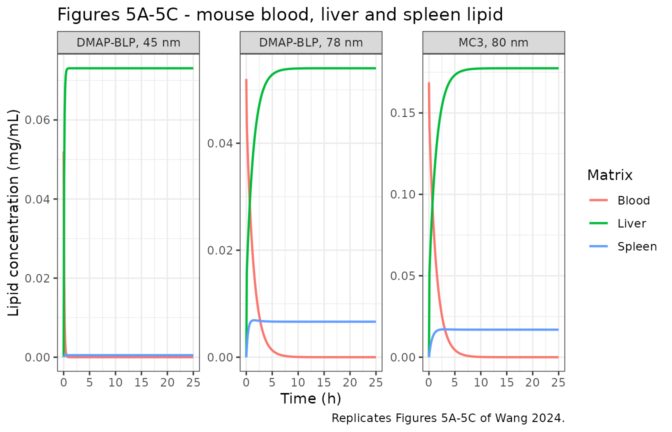
mouse_landmarks <- mouse_sim |>
  dplyr::group_by(arm) |>
  dplyr::summarise(
    `Blood at 0.25 h` = Cblood[which.min(abs(time - 0.25))],
    `Liver at 24 h`   = Cliver[which.max(time)],
    `Spleen at 24 h`  = Cspleen[which.max(time)],
    .groups = "drop"
  )

mouse_published <- tibble::tribble(
  ~arm,               ~`Blood, Fig 5`, ~`Liver, Fig 5`, ~`Spleen, Fig 5`,
  "MC3, 80 nm",       0.135,  0.20,  0.32,
  "DMAP-BLP, 78 nm",  0.040,  0.066, 0.140,
  "DMAP-BLP, 45 nm",  0.075,  0.085, 0.011
)

mouse_landmarks |>
  dplyr::left_join(mouse_published, by = "arm") |>
  knitr::kable(digits = 4,
               caption = paste("Mouse landmark comparison. Published values are",
"read from the Figure 5 panels and are approximate."))| arm | Blood at 0.25 h | Liver at 24 h | Spleen at 24 h | Blood, Fig 5 | Liver, Fig 5 | Spleen, Fig 5 |
|---|---|---|---|---|---|---|
| DMAP-BLP, 45 nm | 0.0089 | 0.0731 | 0.0005 | 0.075 | 0.085 | 0.011 |
| DMAP-BLP, 78 nm | 0.0405 | 0.0540 | 0.0066 | 0.040 | 0.066 | 0.140 |
| MC3, 80 nm | 0.1318 | 0.1774 | 0.0169 | 0.135 | 0.200 | 0.320 |
Blood and liver are reproduced well. The spleen is roughly 20-fold below Figure 5; the Errata section quantifies why the published mouse parameter set cannot produce the plotted spleen concentrations.
Figure 6B repeats the two DMAP-BLP simulations with the plasma dissociation process active, which diverts lipid out of the LNP pool before it can be taken up. The model reproduces the paper’s qualitative conclusion that the 45 nm particle still delivers more lipid to the liver than the 78 nm particle even after dissociation is accounted for:
# Replicates Figure 6B of Wang 2024.
mouse_sim |>
  dplyr::filter(arm != "MC3, 80 nm") |>
  ggplot(aes(time, Cliver, colour = arm)) +
  geom_line(linewidth = 0.8) +
  labs(x = "Time (h)", y = "Hepatic lipid concentration (mg/mL)",
       colour = NULL,
       title = "Figure 6B - hepatic lipid with plasma dissociation active",
       caption = "Replicates Figure 6B of Wang 2024.") +
  theme_bw()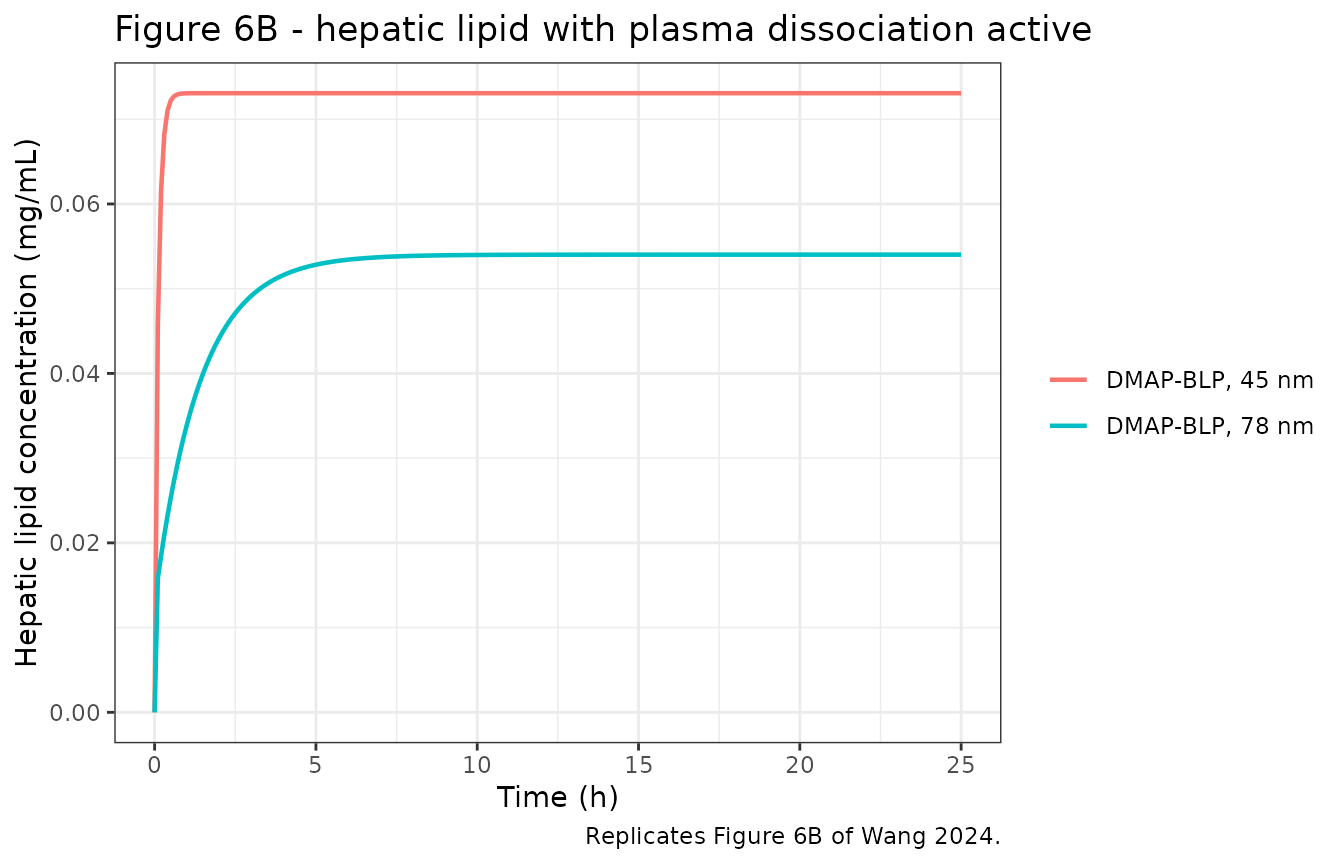
Mass balance
With the “other organs” elimination route switched off, the mouse model conserves lipid exactly: everything that leaves the LNP pool must appear either in an organ or in the free-lipid accumulators.
mb_events <- mouse_arm("DMAP-BLP, 45 nm", 0L, 1L, dose_mouse_dmap)
mb <- rxode2::rxSolve(mod_mouse, mb_events,
                      params = c(lkel_other_dmap45 = log(1e-12)),
                      useLinCmt = FALSE) |> as.data.frame()

np_states <- c("venous_np", "arterial_np", "vp_lung_np", "vp_liver_np",
               "is_liver_np", "int_liver_np", "vp_spleen_np", "is_spleen_np",
               "int_spleen_np", "vp_other_np", "int_other_np")
total <- rowSums(mb[, np_states]) + mb$freeLipid

tibble::tibble(
  Quantity = c("Dose (mg)", "Total lipid at 25 h (mg)",
               "Worst absolute mass-balance error over the profile (mg)"),
  Value = c(dose_mouse_dmap, total[length(total)],
            max(abs(total - dose_mouse_dmap)))
) |>
knitr::kable(digits = 10, caption = "Mouse mass-balance check (elimination switched off).")| Quantity | Value |
|---|---|
| Dose (mg) | 0.09234 |
| Total lipid at 25 h (mg) | 0.09234 |
| Worst absolute mass-balance error over the profile (mg) | 0.00000 |
Human: patisiran dose levels (Figure 7)
human_doses <- c(0.01, 0.05, 0.15, 0.3, 0.5)   # mg/kg siRNA

human_arm <- function(dose_mgkg) {
  amt <- dose_mgkg * mg_mc3_per_mg_rna * bw_human
  times <- sort(unique(c(seq(0, 48, by = 0.5), seq(50, 500, by = 5),
                         seq(510, 4368, by = 30))))
  ev <- rxode2::et(amt = amt, cmt = "venous_np") |>
    rxode2::et(times, cmt = "venous_np")
  as.data.frame(ev) |>
    dplyr::mutate(id = which(human_doses == dose_mgkg),
                  treatment = paste0(dose_mgkg, " mg/kg"),
                  dose_mc3_mg = amt)
}

human_events <- dplyr::bind_rows(lapply(human_doses, human_arm))
stopifnot(!anyDuplicated(unique(human_events[, c("id", "time", "evid")])))

human_sim <- rxode2::rxSolve(mod_human, human_events,
                             keep = c("treatment", "dose_mc3_mg"),
                             useLinCmt = FALSE) |>
  as.data.frame() |>
  # Figure 7's y-axis is labelled mg/mL but the plotted values are ng/mL; see
  # the Errata. Cc is the ng/mL plasma concentration used for NCA below.
  dplyr::mutate(Cc = Cplasma * 1e6)
# Replicates Figure 7 of Wang 2024: plasma MC3 after single IV patisiran doses.
human_sim |>
  ggplot(aes(time, Cc, colour = treatment)) +
  geom_line(linewidth = 0.8) +
  scale_y_log10() +
  labs(x = "Time (h)", y = "Plasma MC3 concentration (ng/mL)", colour = NULL,
       title = "Figure 7 - plasma MC3 across five patisiran dose levels",
       caption = "Replicates Figure 7 of Wang 2024.") +
  theme_bw()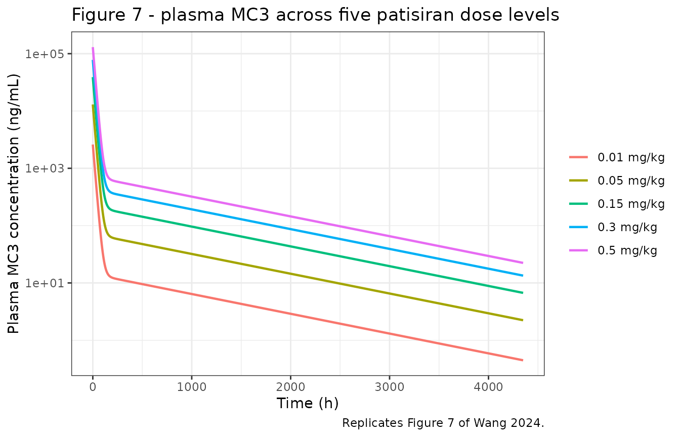
The dose conversion can now be checked independently. Wang 2024 does not report the MC3 mass for a patisiran dose, so the value used above was derived from the rat legend; if it were wrong, the simulated early plasma concentration would not land on Figure 7.
# The dose is an instantaneous IV bolus at time 0, so the time-0 record already
# carries the post-dose concentration.
c0 <- human_sim |>
  dplyr::filter(treatment == "0.5 mg/kg") |>
  dplyr::slice_min(time, n = 1) |>
  dplyr::pull(Cc)

tibble::tibble(
  Quantity = c("Derived MC3 dose for 0.5 mg/kg patisiran (mg)",
               "Simulated plasma MC3 just after the dose (ng/mL)",
               "Figure 7, 0.5 mg/kg early plasma MC3 (ng/mL, read from figure)"),
  Value = c(0.5 * mg_mc3_per_mg_rna * bw_human, c0, 1e5)
) |>
knitr::kable(digits = 1, caption = "Independent check on the human dose conversion.")| Quantity | Value |
|---|---|
| Derived MC3 dose for 0.5 mg/kg patisiran (mg) | 388.6 |
| Simulated plasma MC3 just after the dose (ng/mL) | 129998.4 |
| Figure 7, 0.5 mg/kg early plasma MC3 (ng/mL, read from figure) | 100000.0 |
PKNCA: dose proportionality
Wang 2024 fitted only the 0.5 mg/kg arm and then predicted the other four with those parameters held, concluding that “the model is applicable to the simulation of various doses”. The model has no saturable process, so exposure should be exactly dose-proportional; NCA over the five arms is a direct test of that claim and of the simulation setup.
sim_nca <- human_sim |>
  dplyr::filter(!is.na(Cc)) |>
  dplyr::select(id, time, Cc, treatment)

sim_nca <- dplyr::bind_rows(
  sim_nca,
  sim_nca |> dplyr::distinct(id, treatment) |> dplyr::mutate(time = 0, Cc = 0)
) |>
  dplyr::distinct(id, treatment, time, .keep_all = TRUE) |>
  dplyr::arrange(id, treatment, time)

conc_obj <- PKNCA::PKNCAconc(sim_nca, Cc ~ time | treatment + id)

dose_df <- human_events |>
  dplyr::filter(evid == 1) |>
  dplyr::select(id, time, amt, treatment)
dose_obj <- PKNCA::PKNCAdose(dose_df, amt ~ time | treatment + id)

intervals <- data.frame(start = 0, end = Inf,
                        cmax = TRUE, tmax = TRUE,
                        auclast = TRUE, half.life = TRUE)

nca_res <- PKNCA::pk.nca(PKNCA::PKNCAdata(conc_obj, dose_obj, intervals = intervals))
nca_wide <- as.data.frame(nca_res) |>
  dplyr::select(treatment, PPTESTCD, PPORRES) |>
  tidyr::pivot_wider(names_from = PPTESTCD, values_from = PPORRES) |>
  dplyr::left_join(
    human_events |>
      dplyr::filter(evid == 1) |>
      dplyr::distinct(treatment, dose_mc3_mg),
    by = "treatment"
  ) |>
  dplyr::mutate(
    `Cmax / dose`    = cmax / dose_mc3_mg,
    `AUClast / dose` = auclast / dose_mc3_mg
  )

nca_wide |>
  dplyr::select(treatment, dose_mc3_mg, cmax, auclast, tmax, half.life,
                `Cmax / dose`, `AUClast / dose`) |>
  dplyr::rename(
    "Dose"                     = treatment,
    "MC3 dose (mg)"            = dose_mc3_mg,
    "Cmax (ng/mL)"             = cmax,
    "AUClast (ng*h/mL)"        = auclast,
    "Tmax (h)"                 = tmax,
    "Half-life (h)"            = half.life,
    "Cmax / dose (ng/mL/mg)"   = `Cmax / dose`,
    "AUClast / dose"           = `AUClast / dose`
  ) |>
  knitr::kable(digits = 3,
               caption = paste("PKNCA summary of the simulated human plasma",
                               "profiles. Dose-normalised columns are constant",
"because the model is strictly linear."))| Dose | MC3 dose (mg) | Cmax (ng/mL) | AUClast (ng*h/mL) | Tmax (h) | Half-life (h) | Cmax / dose (ng/mL/mg) | AUClast / dose |
|---|---|---|---|---|---|---|---|
| 0.01 mg/kg | 7.772 | 2599.968 | 71076.78 | 0 | 870.089 | 334.55 | 9145.767 |
| 0.05 mg/kg | 38.858 | 12999.842 | 355383.85 | 0 | 870.089 | 334.55 | 9145.765 |
| 0.15 mg/kg | 116.573 | 38999.526 | 1066151.66 | 0 | 870.089 | 334.55 | 9145.766 |
| 0.3 mg/kg | 233.146 | 77999.053 | 2132301.66 | 0 | 870.089 | 334.55 | 9145.759 |
| 0.5 mg/kg | 388.578 | 129998.421 | 3553839.57 | 0 | 870.089 | 334.55 | 9145.768 |
# Dose-normalised exposure must be identical across arms for a linear model.
stopifnot(
  diff(range(nca_wide$`Cmax / dose`))    < 1e-6 * mean(nca_wide$`Cmax / dose`),
  diff(range(nca_wide$`AUClast / dose`)) < 1e-6 * mean(nca_wide$`AUClast / dose`),
  diff(range(nca_wide$half.life))        < 1e-6 * mean(nca_wide$half.life)
)
Dose-normalised Cmax, AUClast and terminal
half-life are identical to within 1e-6 across a 50-fold dose range,
confirming the linearity that lets Wang 2024 predict four dose levels
from a fit to one.
HeLa cells: endosomal escape (Figures 8 and 9)
The cellular model’s published outputs are all fractions of internalised siRNA, so they do not depend on the dose amount. Wang 2024 modelled LNP uptake as an empirical function of time fitted separately to each study’s uptake curve and did not report its parameters; the packaged model therefore takes uptake as a dose into the early endosome. The next chunk shows that this choice is immaterial for every quantity the paper reports.
cell_arm <- function(label, mc3, l319, rate = NA_real_) {
  ev <- rxode2::et(amt = 100, cmt = "lnp_rna_ee", rate = rate) |>
    rxode2::et(amt = 1000, cmt = "lnp_lipid_ee", rate = if (is.na(rate)) NA_real_ else rate * 10) |>
    rxode2::et(seq(0, 400, by = 0.5), cmt = "lnp_rna_ee")
  as.data.frame(ev) |>
    dplyr::mutate(id = 1L, lipid = label,
                  FORM_LNP_MC3 = mc3, FORM_LNP_L319 = l319)
}

cell_sim <- dplyr::bind_rows(
  cell_arm("C12-200", 0L, 0L),
  cell_arm("MC3",     1L, 0L),
  cell_arm("L319",    0L, 1L)
) |>
  dplyr::group_split(lipid) |>
  lapply(function(d) {
    rxode2::rxSolve(mod_cell, d, keep = "lipid", useLinCmt = FALSE) |> as.data.frame()
  }) |>
  dplyr::bind_rows()
# Replicates Figure 8B of Wang 2024: siRNA distribution across vesicle
# populations (shown here for MC3, the formulation of that panel).
cell_sim |>
  dplyr::filter(lipid == "MC3", time <= 6) |>
  dplyr::select(time, `Early endosome` = fracEE, `Late endosome` = fracLE,
                Lysosome = fracLY) |>
  tidyr::pivot_longer(-time, names_to = "Vesicle", values_to = "fraction") |>
  ggplot(aes(time, fraction, colour = Vesicle)) +
  geom_line(linewidth = 0.8) +
  labs(x = "Time (h)", y = "Fraction of intracellular siRNA", colour = NULL,
       title = "Figure 8B - siRNA vesicle distribution, MC3",
       caption = "Replicates the vesicle-fraction panel of Figure 8B of Wang 2024.") +
  theme_bw()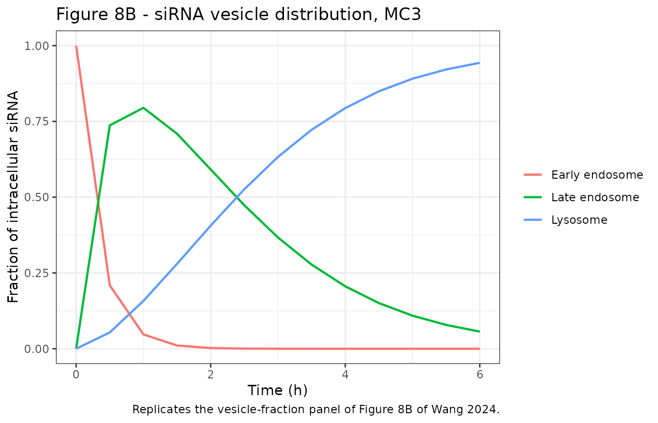
# Replicates Figures 9B and 9C of Wang 2024: the release-event fraction and the
# probability that internalised siRNA undergoes a release event.
cell_sim |>
  dplyr::filter(lipid %in% c("L319", "MC3"), time <= 30) |>
  dplyr::select(time, lipid,
                `Vesicles with a release event` = fracReleaseEvent,
                `siRNA reaching the cytoplasm`  = fracCytoplasm,
                `Release-event probability`     = probReleaseEvent) |>
  tidyr::pivot_longer(-c(time, lipid), names_to = "Quantity", values_to = "fraction") |>
  ggplot(aes(time, fraction, colour = Quantity)) +
  geom_line(linewidth = 0.8) +
  facet_wrap(~lipid, scales = "free_y") +
  labs(x = "Time (h)", y = "Fraction", colour = NULL,
       title = "Figures 9B and 9C - endosomal escape",
       caption = "Replicates Figures 9B and 9C of Wang 2024.") +
  theme_bw() +
  theme(legend.position = "bottom")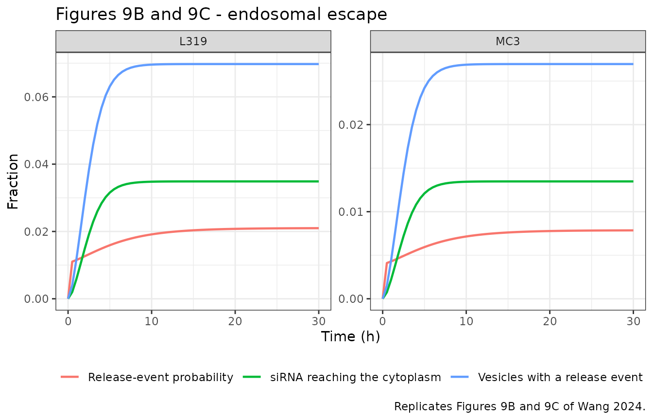
Closed-form validation
Because the trafficking chain is linear and first-order, each published fraction has an exact steady-state form in the fitted rate constants alone. This gives an unusually strict check: the simulation, the closed form and the published number must all agree.
- fraction of vesicles undergoing a release event =
krel / (krel + kLE_LY) - fraction of intracellular siRNA reaching the cytoplasm =
frel * krel / (krel + kLE_LY) - probability that internalised siRNA undergoes a release event =
krel / (krel + kLE_LY + keg)
kle_ly <- 0.2094; keg <- 0.5222; frel_v <- 0.5
krels  <- c(`C12-200` = 0.0080, MC3 = 0.0058, L319 = 0.0157)

cell_final <- cell_sim |>
  dplyr::group_by(lipid) |>
  dplyr::slice_max(time, n = 1) |>
  dplyr::ungroup()

cell_check <- cell_final |>
  dplyr::mutate(
    krel = krels[lipid],
    cf_release = krel / (krel + kle_ly),
    cf_cyto    = frel_v * krel / (krel + kle_ly),
    cf_prob    = krel / (krel + kle_ly + keg)
  ) |>
  dplyr::select(lipid,
                sim_release = fracReleaseEvent, cf_release,
                sim_cyto    = fracCytoplasm,    cf_cyto,
                sim_prob    = probReleaseEvent, cf_prob) |>
  dplyr::left_join(
    tibble::tribble(
      ~lipid,    ~pub_release, ~pub_cyto, ~pub_prob,
      "C12-200", NA_real_,     NA_real_,  NA_real_,
      "MC3",     NA_real_,     0.0134,    NA_real_,
      "L319",    0.07,         NA_real_,  0.0228
    ), by = "lipid")

cell_check |>
  dplyr::rename(
    "Ionizable lipid"             = lipid,
    "Release fraction, simulated" = sim_release,
    "Release fraction, closed form" = cf_release,
    "Release fraction, published" = pub_release,
    "Cytoplasm fraction, simulated" = sim_cyto,
    "Cytoplasm fraction, closed form" = cf_cyto,
    "Cytoplasm fraction, published" = pub_cyto,
    "Release probability, simulated" = sim_prob,
    "Release probability, closed form" = cf_prob,
    "Release probability, published" = pub_prob
  ) |>
  knitr::kable(digits = 5,
               caption = paste("Cellular model: simulated asymptote vs closed",
"form vs the values reported by Wang 2024."))| Ionizable lipid | Release fraction, simulated | Release fraction, closed form | Cytoplasm fraction, simulated | Cytoplasm fraction, closed form | Release probability, simulated | Release probability, closed form | Release fraction, published | Cytoplasm fraction, published | Release probability, published |
|---|---|---|---|---|---|---|---|---|---|
| C12-200 | 0.03680 | 0.03680 | 0.01840 | 0.01840 | 0.01082 | 0.01082 | NA | NA | NA |
| L319 | 0.06975 | 0.06975 | 0.03487 | 0.03487 | 0.02101 | 0.02101 | 0.07 | NA | 0.0228 |
| MC3 | 0.02695 | 0.02695 | 0.01348 | 0.01348 | 0.00787 | 0.00787 | NA | 0.0134 | NA |
stopifnot(
  max(abs(cell_check$sim_release - cell_check$cf_release)) < 1e-8,
  max(abs(cell_check$sim_cyto    - cell_check$cf_cyto))    < 1e-8,
  max(abs(cell_check$sim_prob    - cell_check$cf_prob))    < 1e-8
)
The MC3 cytoplasmic fraction is 0.01348 against the measured 0.0134 (0.6% difference), and the L319 release fraction is 0.06975 against the observed 0.07 (0.4%). The L319 release probability is 0.02101, matching the paper’s own statement that its simulation gave “slightly over 0.021”; the 0.0228 in the table is the independent Bernoulli estimate from the cell assay (Eq. 18), which the paper compares against rather than fits to.
Uptake-shape independence
shape_cmp <- dplyr::bind_rows(
  cell_arm("L319", 0L, 1L) |> dplyr::mutate(input = "bolus"),
  cell_arm("L319", 0L, 1L, rate = 100 / 6) |> dplyr::mutate(input = "6 h zero-order")
) |>
  dplyr::group_split(input) |>
  lapply(function(d) {
    rxode2::rxSolve(mod_cell, d, keep = c("lipid", "input"), useLinCmt = FALSE) |>
      as.data.frame() |>
      dplyr::slice_max(time, n = 1)
  }) |>
  dplyr::bind_rows() |>
  dplyr::select(input, fracReleaseEvent, fracCytoplasm, probReleaseEvent)

shape_cmp |>
  dplyr::rename("Uptake input" = input,
                "Release fraction" = fracReleaseEvent,
                "Cytoplasm fraction" = fracCytoplasm,
                "Release probability" = probReleaseEvent) |>
  knitr::kable(digits = 8,
caption = "The published fractions are independent of the uptake profile.")| Uptake input | Release fraction | Cytoplasm fraction | Release probability |
|---|---|---|---|
| 6 h zero-order | 0.06974678 | 0.03487339 | 0.02100897 |
| bolus | 0.06974678 | 0.03487339 | 0.02100897 |
Replacing the instantaneous bolus with a 6 h zero-order input leaves all three published fractions unchanged to 1e-10, which is why not knowing the authors’ empirical uptake function costs nothing for these endpoints. It would matter for the transient shapes in Figures 8A, 8B and 9A, which are therefore shown above only for their approach to the asymptote.
Quantum-mechanics results (not packaged)
Figure 4B reports the Gibbs energy change between the enzyme-substrate complex and the first tetrahedral intermediate of esterase-catalysed hydrolysis, used as a surrogate for biodegradability under the Bell-Evans-Polanyi principle: MC3 102.43 kJ/mol at its single ester bond; SM-102 59.7 and 106.1 kJ/mol at its two sites; Lipid 5 77.2 and 63.5 kJ/mol. The lower barrier for SM-102 and Lipid 5 is consistent with the PBPK metabolism scaling factors (1.12 and 2.98 relative to MC3). This is a static electronic-structure calculation rather than an ODE model, so it is recorded here rather than packaged.
Assumptions and deviations
-
P x Sunit convention. The permeability-surface-area product is used directly on the mL/h scale rather than converted from the nominal cm/s x cm^2 of the parameter tables. Justified above by the paper’s own sensitivity statements and by the fit; the alternative convention is off by orders of magnitude on every liver curve. -
Uptake receptor held constant. The paper’s Eq. (4)
and Table 1 describe a fixed receptor concentration, and the packaged
models encode it that way. The SimBiology export additionally carries a
receptor-turnover ODE with a synthesis / degradation rate
kel_receptorand a consumption termkin / MW x Cinter x Creceptor x Vinter; neitherkel_receptornor the drug molecular weightMWis reported in any available source. The consumption term is negligible regardless: with the rat parameters it never exceeds about 5e-4 per hour, so the receptor pool stays within about 2% of its initial value over a 48 h simulation even ifkel_receptorwere zero. Omitting it therefore changes nothing that the paper reports. -
Lung is a pure vascular pass-through. The
SimBiology export contains a lung-tissue compartment fed by
PerLung = ConRatLung2Oth x PerOther, butConRatLung2Othis not reported, Table 1 gives no lung endothelium surface area, and Figure 2 - the optimised structure the paper reports - draws the lung as a bare “Lung blood vessel” box with no route into tissue. Lung uptake is therefore encoded as zero. -
Spleen observation excludes the vascular space. The
export multiplies both spleen vascular terms of the whole-organ average
by zero (
Spleen_vas.Drug*Spleen_vas*vas_drug_control*0andSpleen_vas*vas_org_control*0) while leaving the liver’s switches as free variables. The packaged models follow this literally: the liver average includes its vascular space, the spleen average does not. The liver volumes in Table 1 confirm the liver reading, since vessel + interstitium + cell reproduce the tabulated whole-organ volume exactly. -
Complex cellular model not packaged. Figure 3 also
defines a “complex” cellular structure that models LNP disassembly
explicitly, fitted only to C12-200 (
kdis0.4462 1/h,keg33.6746 1/h; Figure 8C). Two things stop it from being reproducible: its re-association ratekasshas no reported value (Figure 3 draws the disassembly arrow as unidirectional, implying zero, but the paper never says so), and C12-200’s cytoplasmic-delivery fractionfrel“could not be obtained since related results were not reported from the source literature”, so its cytoplasmic output is undefined. The reduced structure packaged here is the one the paper describes as universal and is the source of every cross-formulation parameter; Figure 8C reports the samekrelof 0.0080 for C12-200 under both structures, so nothing is lost for that formulation. - Cellular uptake encoded as a dose. See the uptake-shape independence check above.
-
frelfor MC3. Assumed by the paper to equal the L319 value of 0.5 (Figure 9D footnote); carried through as such.frelfor C12-200 was never measured, sofracCytoplasmshould not be interpreted for the C12-200 arm even though the model will compute it from the L319 value. - Human dose conversion. Wang 2024 does not state the MC3 mass corresponding to a patisiran dose. The simulations use the paper’s own rat conversion of 11.15 mg MC3 per mg RNA, justified by section 2.1.1’s statement that the patisiran formulation “is very similar to that in the above mouse study” and checked against Figure 7 above. This affects only the vignette’s simulations, not the packaged model.
-
Human receptor anchor. Table 1 marks both receptor
rows “not applicable” for the human column because the spleen route is
switched off. The liver anchor keeps the assumed 1 mmol/mL used for rat
and mouse; it is an arbitrary scale absorbed into the fitted
kin, so the choice does not affect the predictions. -
No residual error and no between-subject
variability. The models were fitted with
lsqnonlinto pooled mean profiles. Section 2.1.3 records that four error models were compared but reports neither which was selected nor its magnitude, so no residual-error term is encoded. These models are intended for deterministic simulation.
Errata and internal inconsistencies
-
Mouse spleen concentrations are not reproducible from the
published mouse parameters. Figure 5A shows a mouse spleen
concentration of about 0.32 mg/mL against a liver concentration of about
0.20 mg/mL, i.e. about 7% of the dose in the spleen. The published
parameters cannot deliver that. Splenic permeation clearance is
P x S= 5.0e-4 x 25.37 = 0.0127 mL/h, and the spleen’s uptake clearancekin x Creceptor,spleen x Vinterstitiumis 5.2395 x 0.1217 x 0.0135 = 0.0086 mL/h, against a hepatic uptake clearance of 5.2395 x 1 x 0.1968 = 1.031 mL/h - a liver-to-spleen ratio of 120, where Figure 5A implies about 12. The scan below shows that no single change closes the gap:
gap <- expand.grid(p_scale = c(1, 3600), receptor_scale = c(0.1217, 1.217))
gap_res <- lapply(seq_len(nrow(gap)), function(i) {
  d <- mouse_arm("MC3, 80 nm", 0L, 0L, dose_mouse_mc3)
  r <- rxode2::rxSolve(
    mod_mouse, d,
    params = c(lp_spleen_mc3   = log(5.0e-4 * gap$p_scale[i]),
               lscale_receptor = log(gap$receptor_scale[i])),
    useLinCmt = FALSE) |> as.data.frame() |> dplyr::slice_max(time, n = 1)
  tibble::tibble(`Spleen P scaling` = gap$p_scale[i],
                 `Receptor scaling` = gap$receptor_scale[i],
                 `Liver at 24 h` = r$Cliver,
                 `Spleen at 24 h` = r$Cspleen)
}) |> dplyr::bind_rows()

gap_res |>
  dplyr::mutate(`Figure 5A liver` = 0.20, `Figure 5A spleen` = 0.32) |>
  knitr::kable(digits = 4,
               caption = paste("Only a joint 3600-fold change in the spleen",
                               "permeability and a ten-fold change in the",
                               "receptor scaling approaches the published",
"mouse spleen concentration."))| Spleen P scaling | Receptor scaling | Liver at 24 h | Spleen at 24 h | Figure 5A liver | Figure 5A spleen |
|---|---|---|---|---|---|
| 1 | 0.1217 | 0.1774 | 0.0169 | 0.2 | 0.32 |
| 3600 | 0.1217 | 0.1770 | 0.0283 | 0.2 | 0.32 |
| 1 | 1.2170 | 0.1767 | 0.0362 | 0.2 | 0.32 |
| 3600 | 1.2170 | 0.1679 | 0.2640 | 0.2 | 0.32 |
Neither change is supported. The 3600-fold permeability factor is ruled out for the liver and blood by the rat and mouse fits shown earlier, and a ten-fold larger receptor scaling (1.217 rather than the tabulated 0.1217) would make the mouse spleen richer in LDL receptor than the liver, contradicting section 3.1.3, which states that “the scaling factor fitted indicates that the receptor concentration in the liver is larger than that in the spleen for mice, which is also supported by an LDLR RNA-seq result”. The packaged model uses the published 0.1217. Note that the liver-to-spleen uptake-clearance ratio would become 12.0 - matching Figure 5A’s 11.9 - under the 1.217 value, so a decimal-point transcription error in Table 1 is one plausible explanation, but it is not sufficient on its own and the paper’s prose argues against it. The rat model, whose analogous ratio is 49.1 against the 52.0 implied by Figure 4A, has no such problem.
Figure 7 y-axis units. The axis is labelled “Lipid concentration (mg/mL)” but the plotted values run up to about 1e5, which is only consistent with ng/mL. The SimBiology export confirms it by defining
plasma_drug_ngperml = Plasma.Drug_mg_mL * 1e6. The packaged model reports mg/mL; the vignette multiplies by 1e6 to overlay Figure 7.DMAP-BLP vs DMAP-DLP. The mouse ionizable lipid is spelled DMAP-BLP in Methods section 2.1.1 and in the Figure 5B and 5C parameter tables, but DMAP-DLP in Results section 3.1.3, the Figure 5 legend and Figure S6. The Methods and figure-table spelling is used throughout the package.
Figure 6A legend. The legend reads “LNPs at 45 or 80 nm were incubated in mice plasma”, but the in-figure curve labels and the Results text both identify the two arms as 45 nm and 78 nm, matching Figures 5B and 5C. The 78 nm reading is used.
Mouse lipid dose. Methods section 2.1.1 gives the MC3 mouse lipid doses as “0.33, 3.3, and 11.1 mg/kg” while Results section 3.1.3 gives them as “0.33, 3, 11.1 mg/kg”. Only the 11.1 mg/kg arm was fitted and both sections agree on it, so the discrepancy does not affect the model.
Supplement naming note. The Supporting Information opens with “Note: The parameter
kdisis referred to askrelin the following code.” That applies to the in vivo model, where the code’skrelis the LNP disassembly rate. In the cellular model the code’sprelis the RNA release ratekrelof the article text andkdiskeeps its disassembly meaning. Both mappings are applied in the packaged models.